the Creative Commons Attribution 4.0 License.
the Creative Commons Attribution 4.0 License.
 | 27 Apr 2018
Nonlinear analysis of the occurrence of hurricanes in the Gulf of Mexico and the Caribbean Sea
Berenice Rojo-Garibaldi
David Alberto Salas-de-León
María Adela Monreal-Gómez
Norma Leticia Sánchez-Santillán
David Salas-Monreal
Hurricanes are complex systems that carry large amounts of energy. Their impact often produces natural disasters involving the loss of human lives and materials, such as infrastructure, valued at billions of US dollars. However, not everything about hurricanes is negative, as hurricanes are the main source of rainwater for the regions where they develop. This study shows a nonlinear analysis of the time series of the occurrence of hurricanes in the Gulf of Mexico and the Caribbean Sea obtained from 1749 to 2012. The construction of the hurricane time series was carried out based on the hurricane database of the North Atlantic basin hurricane database (HURDAT) and the published historical information. The hurricane time series provides a unique historical record on information about ocean–atmosphere interactions. The Lyapunov exponent indicated that the system presented chaotic dynamics, and the spectral analysis and nonlinear analyses of the time series of the hurricanes showed chaotic edge behavior. One possible explanation for this chaotic edge is the individual chaotic behavior of hurricanes, either by category or individually regardless of their category and their behavior on a regular basis.


Hurricanes have been studied since ancient times, and their activity is related to disasters and loss of life. In recent years, there has been considerable progress in predicting their trajectory and intensity once tracking has begun, as well as their number and intensity from one year to the next. However, their long-term and very short-term prediction remains a challenge (Halsey and Jensen, 2004), and the damage to both materials and lives remains considerable. Therefore, it is important to make a greater effort regarding the study of hurricanes in order to reduce the damage they cause. The periodic behavior of hurricanes and their relationships with other natural phenomena have usually been performed with linear-type analyzes, which have provided valuable information. However, we decided to make a different contribution by carrying out a nonlinear analysis of a time series of hurricanes that occurred in the Gulf of Mexico and the Caribbean Sea, as the dynamics of the system are controlled by a set of variables of low dimensionality (Gratrix and Elgin, 2004; Broomhead and King, 1986).
One of the core sections of this work was the elaborate time series that was built, especially for the oldest part of the registry, for which it was possible to compile a substantial and robust collection. This provided our time series with an amount of data with which it was possible to perform the desired analysis; otherwise, it would have been impossible to study this natural phenomenon via nonlinear analysis.
Different methods have been used in the analysis of non-linear, non-stationary and non-Gaussian processes, including artificial neural networks (ASCE Task Committee, 2000; Maier and Dandy, 2000; Maier et al., 2010; Taormina et al., 2015). Chen et al. (2015) use a hybrid neural network model to forecast the flow of the Altamaha River in Georgia; Gholami et al. (2015) simulate groundwater levels using dendrochronology and an artificial neural network model for the southern Caspian coast in Iran. Furthermore, theories of deterministic chaos and fractal structure have already been applied to atmospheric boundary data (Tsonis and Elsner, 1988; Zeng et al., 1992), e.g., to the pulse of severe rain time series (Sharifi et al., 1990; Zeng et al., 1992) and to tropical cyclone trajectory (Fraedrich and Leslie, 1989; Fraedrich et al., 1990). Natural phenomena occur within different contexts; however, they often exhibit common characteristics, or may be understood using similar concepts. Deterministic chaos and fractal structure in dissipative dynamical systems are among the most important nonlinear paradigms (Zeng et al., 1992). For a detailed analysis of deterministic chaos, the Lyapunov exponent is utilized as a key point and several methods have been developed to calculate it. It is possible to define different Lyapunov exponents for a dynamic system. The maximal Lyapunov exponent can be determined without the explicit construction of a time-series model. A reliable characterization requires that the independence of the embedded parameters and the exponential law for the growth of distances can be explicitly tested (Rigney et al., 1993; Rosenstein et al., 1993). This exponent provides a qualitative characterization of the dynamic behavior and the predictability measurement (Atari et al., 2003). The algorithms usually employed to obtain the Lyapunov exponent are those proposed by Wolf (1986), Eckmann and Ruelle (1992), Kantz (1994) and Rosenstein et al. (1993). The methods of Wolf (1986) and Eckmann and Ruelle (1992) assume that the data source is a deterministic dynamic system and that irregular fluctuations in time-series data are due to deterministic chaos. A blind application of this algorithm to an arbitrary set of data will always produce numbers, i.e., these methods do not provide a strong test of whether the calculated numbers can actually be interpreted as Lyapunov exponents of a deterministic system (Kantz et al., 2013). The Rosenstein et al. (1993) method follows directly from the definition of the Lyapunov maximal exponent and is accurate because it takes advantage of all available data. The algorithm is fast, easy to implement and robust to changes in the following quantities: embedded dimensions, data set size, delay reconstruction and noise level. The Kantz (1994) algorithm is similar to that of Rosenstein et al. (1993).
We constructed a database of occurrences of hurricanes in the Gulf of Mexico and the Caribbean Sea to perform a nonlinear analysis of the time series, the results from which can aid in the construction of hurricane occurrence models, which in turn will help to reinforce prevention measures for this type of hydrometeorological phenomenon.
2.1 Data set description
A detailed analysis of historical reports was carried out in order to obtain the annual time series of hurricane occurrence, from category one to five on the Saffir–Simpson scale, in the study region from 1749 to 2012. The time series was composed using the historical ship track of all vessels sailing close to registered hurricanes, the aerial reconnaissance data for hurricanes since 1944 and the hurricanes reported by Fernández-Partagas and Díaz (1995a, b, 1996a, b, c, 1997, 1999). All of the abovementioned information in addition to the database of the HURDAT re-analysis project (HURDAT is the official record of the United States for tropical storms and hurricanes occurring in the Atlantic Ocean, the Gulf of Mexico and the Caribbean Sea) was used in a comparative way in order to build our time series (Fig. 1), which is currently the longest time series of hurricanes for the Gulf of Mexico and the Caribbean Sea. This makes our series ideal for performing a nonlinear analysis, which would be impossible with the records available in other regions.

Figure 1Hurricanes between 1749 and 2012. The dashed line shows the linear trend (after Rojo-Garibaldi et al., 2016).
Historical hurricanes were included only if they were reported in two or more databases and met both of the following criteria: the reported hurricanes that touched land and those that remained in the ocean; on the other hand, the followed hurricanes were studied considering their average duration and their maximum time (9 and 19 days, respectively). This was done in order to avoid counting more than one specific hurricane reported in different places within a short period time; to do this, we followed the proposed method by Rojo-Garibaldi et al. (2016).

Figure 2Phase diagrams corresponding to the time series of hurricanes that occurred between 1749 and 2012 in the Gulf of Mexico and the Caribbean Sea. The x axis in the four plots indicates the time lag (τ).
2.2 Data reduction and procedures
Before performing the nonlinear analysis of the time series, we removed the trend; thus, the series was prepared according to what is required for this type of analysis. To uncover the properties of the system, however, requires more than just estimating the dimensions of the attractor (Jensen et al., 1985); therefore, three methods were applied in this study:
-
The Hurst exponent is a measure of the independence of the time series as an element to distinguish a fractal series. It is basically a statistical method that provides the number of occurrences of rare events and is usually called re-scaling (RS) rank analysis (Gutiérrez, 2008). According to Miramontes and Rohani (1998), the Hurst exponent also provides another approximation that can be used to characterize the color of noise, and could therefore be applied to any time series. The RS helps to find the Hurst exponent, which provides the numerical value which makes it possible to determine the autocorrelation in a data series.
-
The Lyapunov exponent is invariant under soft transformations, because it describes long-term behavior, providing an objective characterization of the corresponding dynamics (Kantz and Schreiber, 2004). The presence of chaos in dynamic systems can be solved using this exponent, as it quantifies the exponential convergence or divergence of initially close trajectories in the state space and estimates the amount of chaos in a system (Rosenstein et al., 1993; Haken, 1981; Wolf, 1986). The Lyapunov exponent (λ) can take one of the following four values: λ < 0, which corresponds to a stable fixed point; λ = 0, which is for a stable limit cycle; 0 < λ < ∞, which indicates chaos; and λ=∞, a Brownian process, which agrees with the fact that the entropy of a stochastic process is infinite (Kantz and Schreiber, 2004).
-
The iterated function analysis (IFS) is an easier and simpler way to visualize the fine structure of the time series because it can reveal correlations in the data and help to characterize its color, referring color to the type of noise (Miramontes et al., 2001). Together with the Lyapunov exponent, the phase diagrams, the false close neighbors method, the space-time separation plot, the correlation integral plot and the correlation dimension were taken into account, the latter two to identify whether the system attractor was a fractal type or not. It is important to compute the Lyapunov exponent, so we used the algorithms proposed by Kantz (1994) and Rosenstein et al. (1993) to do so.
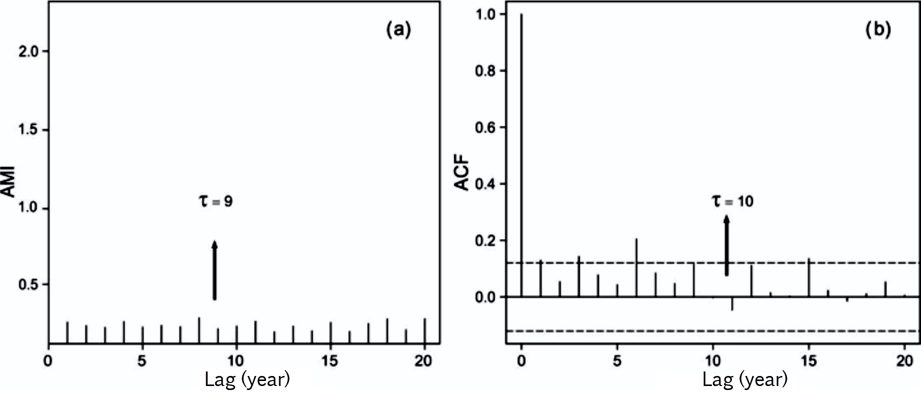
Figure 3The mutual information method (a): the x axis indicates the time lag against the mutual information index (AMI) and the arrow indicates the first, most pronounced minimum with a value of τ = 9. The autocorrelation function (b), the x axis indicates the time lag versus the value of the autocorrelation function, and the arrow denotes where the first zero of the function τ = 10 was obtained.
Figure 1 shows the evolution of the number of hurricanes from 1749 to 2012 and the linear trend. To have a qualitative idea of the behavior of the number of hurricanes that occurred in the Gulf of Mexico and the Caribbean Sea from 1749 to 2012, a phase diagram was created using the ”delay method” (Fig. 2). This was also used to elucidate the time lag for an optimal embedding in the data set. The optimal time lag (τ) obtained visually from Fig. 2 was equal to nine, since it was the time in which the curves of the system were better divided. We must not forget that this was only a visual inspection, and the delay time is obtained quantitatively by other methods. In our case, the hurricane dynamics were not distinguished through the phase diagram; however, as any hurricane trajectory starts at a close point location on the attractor data set which diverges exponentially, the phase diagram is a primary evidence of a chaotic motion according to Thompson and Stewart (1986).
The most robust method to identify chaos within the system is the Lyapunov exponent. Prior to obtaining the exponent, it was necessary to calculate the time lag and the embedding dimension, and for the latter, the Theiler window was used. The time lag was obtained via three different methods:
-
The method of constructing delays, which is observed visually in Fig. 2.
-
The method of mutual information, which yields a more reliable result as it takes nonlinear dynamic correlations into account; in this study, the delay time was obtained by taking the first minimum of the function – in this case τ=9.
-
The autocorrelation function method, which is based solely on linear statistics (Fig. 3).
There are two ways to obtain the time lag from the autocorrelation function:
-
the first zero of the function, and
-
the moment in which the autocorrelation function decays as 1∕e (Kantz and Schreiber, 2004).
We used the criterion of the first zero because the Hurst exponent (H=0.032) indicated that it was a short memory process; therefore, the criterion of the first zero is the optimal method in this type of case. Using this method, the value that was obtained was τ = 10. The value of this parameter is very important, because if it turns out to be very small, then each coordinate is almost the same and the reconstructed trajectories look like a line (the phenomenon is known as redundancy). If the delay time is quite large, however, then due to the sensitivity of the chaotic movement, the coordinates appear to be independent and the reconstructed phase space looks random or complex (a phenomenon known as irrelevance) (Bradley and Kantz, 2015).

Figure 4False close neighbors with a time lag of 10, where the embedding dimension of 5 has a 9.4 % and the embedding dimension of 4 has a 16.66 % false close neighbors (lower line). False close neighbors with a time lag of 9, where the embedding dimension of 5 has a 20.15 % and the embedding dimension of 4 has a 20.12 % false close neighbors (upper line). The values in each line indicate the optimal dimension for each lag.
The Hurst exponent helps us to identify the criteria to find a time lag, and also describes the system behavior (Quintero and Delgado, 2011). This could indicate that the system does not have chaotic behavior; however, the remaining methods have indicated the opposite, and as previously mentioned, the Lyapunov exponent is considered the most appropriate method for this type of data set. Therefore, different methods will provide different results, but the time series will indicate the best method and the result we should use.
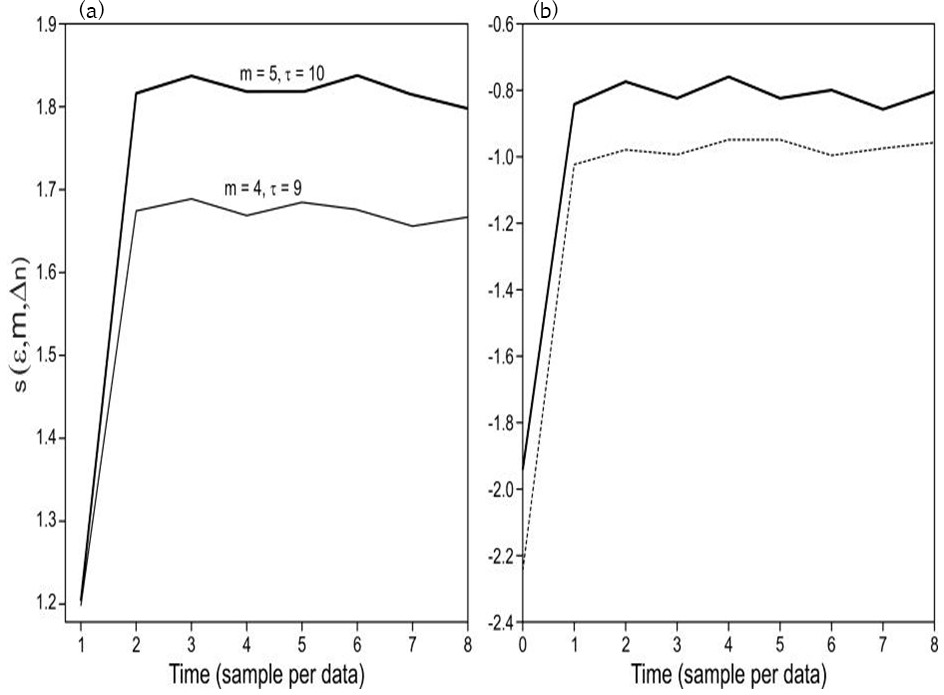
Figure 5Lyapunov exponent with m = 4, τ = 9 and m = 5, τ = 10, with the Kantz method (a). Lyapunov exponent with the same values with the Rosenstein method (b).
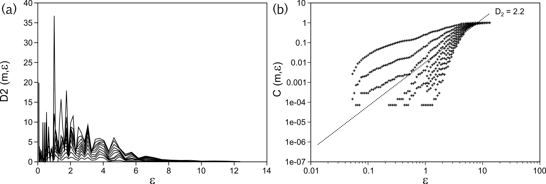
Figure 6The correlation dimension D2 corresponding to the occurrence of hurricanes in the years 1749–2012 in the Gulf of Mexico and the Caribbean Sea. Curves for different dimensions of the attractor (y axis) (a). Same information for the D2 with a logarithmic scale on the x axis (b),
It was possible to observe the difference in the time lag obtained through the autocorrelation function and the mutual information; however, it is necessary to use only one result. Through the space-time separation graphic and the false close neighbors method, we obtained embedding dimensions of m=4 for a τ = 9 and m=5 for τ = 10, and the Theiler window with a value of W = 16 for τ = 9 and W = 18 for τ = 10 (Fig. 4). The choice of this window is very important so as not to obtain subsequent spurious dimensions in the attractor. According to Bradley and Kantz (2015), the Theiler window ensures that the time spacing between the potential pairs of points is large enough to represent a distributed sample identically and independently.
The idea of the false close neighbors algorithm is that at each point in the time series, and its neighbor should be searched in a m-dimensional space. Thus, the distance ∥St−Sj∥ is calculated iterating both points, given by the following:
If Ri is greater than the threshold given by Rt, then SJ has false close neighbors. According to Kennel et al. (1992), a value of Rt = 10 has proven to be a good choice for most data sets, but a formal mathematical proof for this conclusion is not known; therefore, if this value does not give convincing results, it is advisable to repeat the calculations for several Rt (Perc, 2006). In our case, this value gave relevant results. It may have some false close neighbors even when working with the correct embedding dimension. The result of this analysis may depend on the time lag (Kantz and Schreiber, 2004). In a similar fashion to the delay time, the value of the embedment dimension is crucial not only for the reconstruction of the phase space but also to obtain the Lyapunov exponent. Choosing a large value of m for chaotic data will add redundancy and consequently affect the development of many algorithms such as the Lyapunov exponent (Kantz and Schreiber, 2004).
The Lyapunov (λ) exponents were obtained using the Kantz and Rosenstein methods and took the time lag, the embedding dimension and the Theiler window as the main values; however, an election of the neighborhood radius for the exploration of trajectories was also made, as well as the points of reference and the neighbors near these points. The modification of these parameters is important to corroborate the invariant characteristic of the Lyapunov exponent. The Kantz (1994) method using a value of m=4 and τ = 9 gave us an exponent of λ = 0.483, while for m=5 and τ = 10 the exponent was λ = 0.483. As λ is a positive value, it was inferred that our system is chaotic. In addition, the value of λ obtained for both imbibing dimensions was the same, suggesting that our result is accurate. Using the Rosenstein et al. (1993) method, the value obtained for m=4 and τ=9 was λ = 0.1056, and for m=5 and τ = 10, the exponent was λ = 0.112 (Fig. 5).
There was a difference between placing the attractor in an embedding dimension of m=4 and one of m= 5; a better unfolding of the attractor in the embedding dimension was observed in m=4 and τ = 9. This value of τ was obtained with the mutual information method, which, according to Fraser and Swinney (1986) and Krakovská et al. (2015), provides a better criterion for the choice of delay time than the value obtained by the autocorrelation function.
It was possible to obtain the correlation dimension D2 (Fig. 6) and the correlation integral (Fig. 6) using the embedding dimension, the delay time and the Theiler window, following the method of Grassberger and Procaccia (1983a, 1983b). This was done in order to obtain the possible dimensions of the attractor. It should be noted that there is a whole family of fractal dimensions, which are usually known as Renyi dimensions, but these are based on the direct application of box-counting methods, which demands significant memory and processing and the results of which can be very sensitive to the length of the data (Bradley and Kantz, 2015). That is why we chose to use the dimension and integral correlation, which according to Bradley and Kantz (2015) is a more efficient and robust estimator.
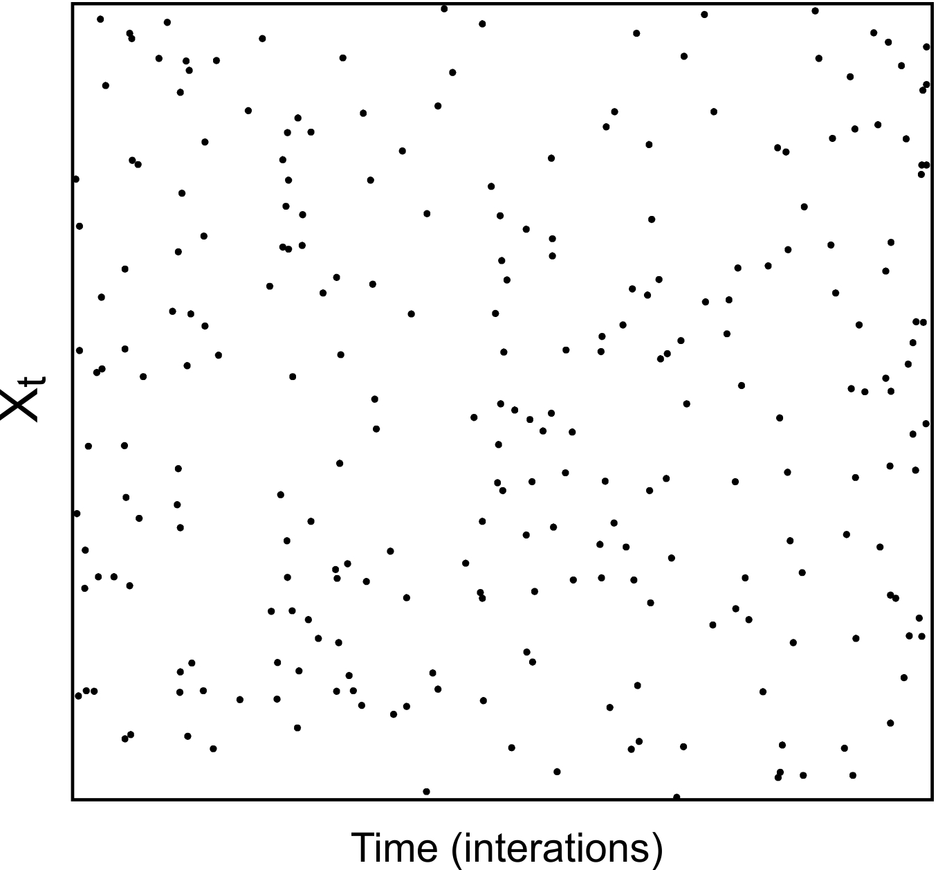
Figure 7The iterated functions system (IFS) test applied to the time series of the number of hurricanes that occurred in the Gulf of Mexico and the Caribbean Sea between the years 1749 and 2012.
The right panel on Fig. 7 shows the slope trend of the majority of the slopes of the correlation integral (ε). In the range of 1 < ε < 10, we are required to have straight lines as an indicator of the self-similar geometry. The value obtained here corresponds to D2=2.20 which is the aforementioned slope value. Another method to see the attractor dimension is the Kaplan–Yorke dimension (DKY), which is associated with the spectrum of Lyapunov exponents and is given by the following:
where k is the maximal integer, such that the sum of the k major exponents is not negative. The fractal dimension with this method yielded a value of DKY = 2.26, which is similar to the one obtained previously.
Even when all the requirements necessary to apply the nonlinear analysis to our time series are present, one final requirement must be fulfilled to know whether we can obtain a dimension and whether the complete spectrum of Lyapunov exponents (another method to visualize chaos) still needs to be employed.
Eckmann and Ruelle (1992) discuss the size of the data set required to estimate Lyapunov dimensions and exponents. When these dimensions and exponents measure the divergence rate with near-initial conditions, they require a number of neighbors for a given reference point. These neighbors may be within a sphere of radius (r) and of a given diameter (d) of the reconstructed attractor.
We then have the requirements for the Eckmann and Ruelle (1992) condition to obtain the Lyapunov exponents as
where D is the dimension of the attractor, N is the number of data points and . For ρ=0.1 in Eq. (3), N may be chosen such that
Our time series met this requirement; therefore, it supports our previous results.
The attractor dimension was mainly obtained because this value tells us the number of parameters or degrees of freedom necessary to control or understand the temporal evolution of our system in the phase space and helps us to determine how chaotic our system is. Using the previous methods, a final fractal dimension of D2 = 2.2 was obtained. Following the embedding laws, it stands to reason that m>D2 (Sauer and Yorke, 1993; Kantz and Schreiber, 2004; Bradley and Kantz, 2015). The criterion of Ruelle (1990) was used to corroborate that the obtained dimension of the attractor is reliable, where ; once the data fulfill this requirement, we can say that the dimension of the attractor is reliable. Finally, the results indicated that at least three parameters are needed to characterize our system, since the 2.2 dimension indicates that the attractor dimension falls between two and three.
The spectrum of the Lyapunov exponent gives 0.09983, −0.07443, −0.23387 and −0.73958; therefore, the total sum is , and according to the previous theory, it is enough have at least one positive exponent in the spectrum of our system in order to have chaotic behavior. Finally, the total sum of the spectrum of Lyapunov exponents was negative, indicating that there is a stable attractor, as mentioned previously. However, since the stable attractor was not easily distinguished, we used a final method in order to confirm if our system presented some chaotic dynamic behavior. This method comprised the iterated functions system test (IFS) (Fig. 7).
Using Fig. 7, it can be observed that the points representing our system occupy the entire space; according to the IFS test, there are two possible explanations:
-
The distribution belongs to a white noise signal and in systems without experimental noise, the point distribution gives a single curve (Jensen et al., 1985). However, the previous Hurst exponent obtained was not equal to zero; therefore, the white noise was also discarded with the autocorrelation function.
-
The system is chaotic with high dimensionality. So far, our results have converged on the occurrence of hurricanes in the Gulf of Mexico and the Caribbean Sea being a chaotic system, so it is feasible to adopt the second explanation. Conversely however, our Lyapunov exponent figure was not flat and it did not seem to flatten as the dimension of embedding increased, which, according to Rosenstein et al. (1993), would mean that our system is not chaotic; although the Lyapunov exponent increased with the decrease in the embedment dimension, which is, again, a characteristic of chaotic systems. It was then also possible to obtain a dimension of the attractor and a positive Lyapunov exponent.
Our results were not easy to interpret because the series presented certain periodic characteristics in an oscillatory fashion and simultaneously showed chaotic behavior. According to Rojo-Garibaldi et al. (2016), the series of hurricanes which had spectral analyzes carried out presented strong periodicities that correspond to sunspots, which are believed to have caused the periodic behavior mentioned above. According to Zeng et al. (1990), the spectral power analysis is often used to distinguish a chaotic or quasi-periodic behavior of periodic structures and to identify different periods embedded in a chaotic signal. Although, as Schuster (1988) and Tsonis (1992) mention, the power spectrum is not only characteristic of a process of deterministic chaos but also of a linear stochastic process. In our case, this behavior was not observed in the spectra obtained, which allowed us to detect periodic signals. The spectra identify two types of behavior in our system. On one hand, there are periodic behaviors associated with external forcing, such as the sunspot cycle, giving the system sufficient order to develop; whilst on the other hand, external forcing presents a chaotic behavior, which gives the system a certain disorder and allows it to be able to adapt to new changes and evolve. The IFS test showed that the occurrence of hurricanes in the Gulf of Mexico and the Caribbean Sea is chaotic with high dimensionality. Fraedrich and Leslie (1989) analyzed the trajectories of cyclones in the region of Australia and calculated the dimensionality of this process, obtaining a result of between six and eight, i.e., a chaotic process of high dimensionality, which is similar to what we find with the IFS method. Halsey and Jensen (2004) furthermore postulate that hurricanes contain a large number of dimensions in phase space.
One possible explanation is localized within a boundary where chaos and order are separated; this boundary is commonly known as the ”edge of chaos” (Langton, 1990; Miramontes et al., 2001). Miramontes et al. (2001) found this type of behavior in ants of the genus Leptothorax, when studying them individually and in groups. In the former, the behavior was periodic, whilst in the latter, the behavior was chaotic. In our case, we believe that the chaotic behavior is due to the individual behavior or the hurricane category, as the high dimensionality suggested by the IFS test agrees with the high dimensionality reported by Fraedrich and Leslie (1989) obtained by studying the trajectories of cyclones – that is, by studying them individually – while the periodic response is due to the behavior of hurricanes as a whole.
Finally, an entropy test was performed using non-linear methods and locally linear prediction (making the prediction at one step), with both methods showing a predictability value of 2.78 years. The locally linear prediction method was applied as follows: the last known state of the system, represented by a vector x = [x(n), x(n+τ),…, x(n + (m−1) τ)], was determined, where m is the embedment dimension and τ is the delay time. We then found the p nearby states (usually close neighbors of x) of the system which represent what has happened in the past, these were obtained by calculating their distances to x. The idea is then to adjust a map that extrapolates x and its neighboring p to determine the following values (Dasan et al., 2002). Based on the above, the value of the embedding dimension and the delay time were changed. Different values of m were used in order to elucidate the most accurate result; this was obtained with a dimension of m = 4 and τ = 9, which are the values for which the attractor of the system was obtained. Therefore, a good prediction is possible until (Fig. 8). Furthermore, if we get away from the measured data (reported hurricanes) the uncertainty grows in an oscillatory way. For the first two data (2013 and 2014), the absolute error in the prediction (observed value – predicted) is less than 0.2, for the third and fourth value (2015 and 2016) it is between 0.2 and 0.3 and for 2017 the error is much greater and gives an overestimation of one hurricane (Fig. 8). An important result of this study is that it allows one to establish the predictability range of a system.
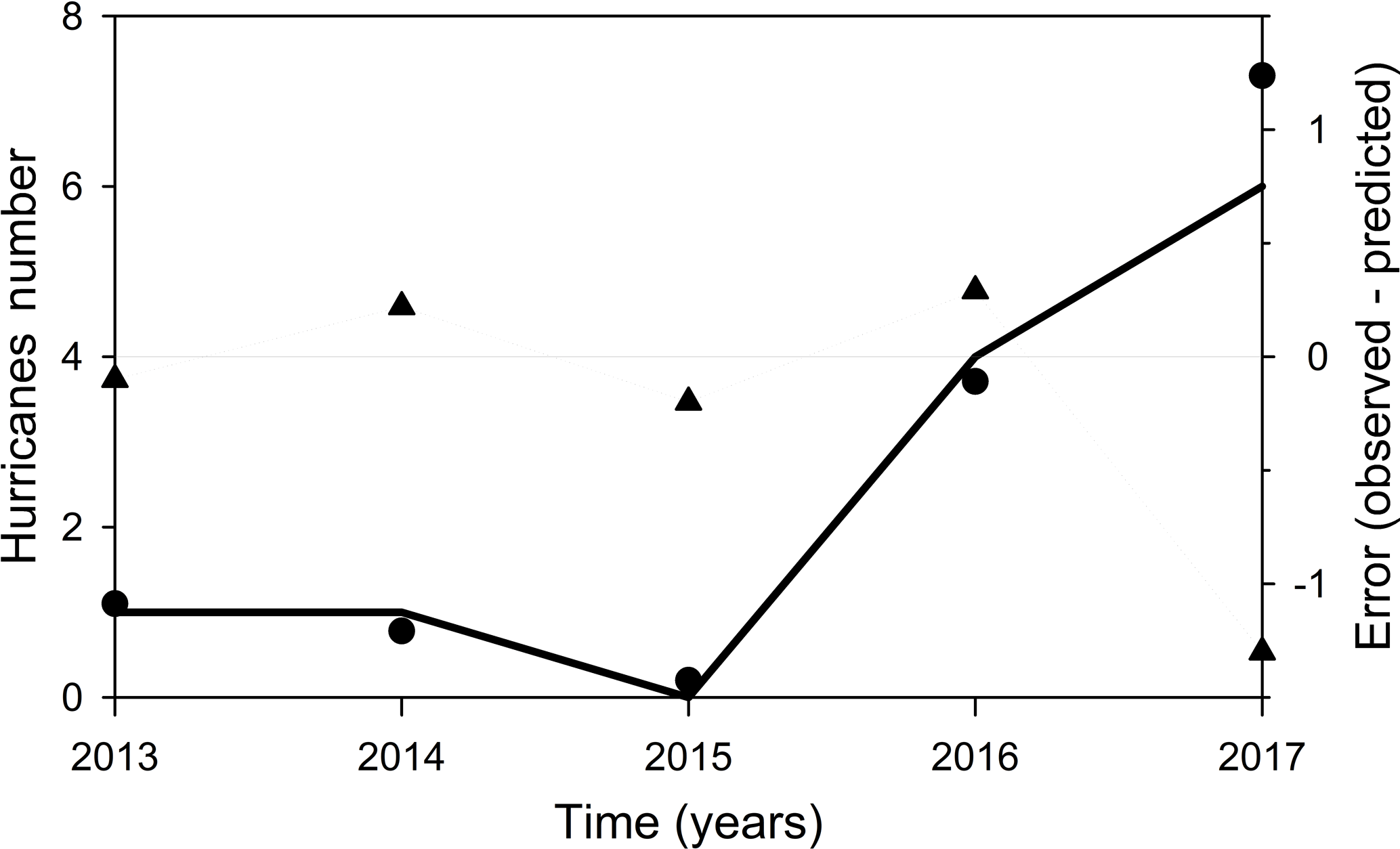
Figure 8Prediction of the hurricanes number in the Gulf of Mexico and the Caribbean Sea by means of non-linear methods, and the entropy test. The solid black line represents the number of hurricanes observed from 2013 to 2017. The black points are the prediction and the triangles are the error in the prediction, considered as the observed values minus the predicted values.
The results obtained with the nonlinear analysis suggested a chaotic behavior in our system, mainly based on the Lyapunov exponents and correlation dimension, among others. However, the Hurst exponent indicated that our system did not follow a chaotic behavior. In order to be able to corroborate our results, we employed the IFS method, which led us to believe that the hurricane time series in the Gulf of Mexico and the Caribbean Sea from 1749 to 2012 had a chaotic edge. It is important to emphasize that this study was prepared as an attempt at understanding the behavior of the occurrence of hurricanes from a historical perspective, as this type of phenomenon is part of an ocean–atmosphere interaction that has been changing over time, hence the value of our contribution. However, we are aware that from the time the study was conducted to the present date there are new records, which will make it possible to carry out new studies and apply new methods.
The data are available upon request from the author.
All the authors contributed equally to this work.
The authors declare that they have no conflict of interest.
This work was financially supported by the Instituto de Ciencias del Mar y
Limnología de la Universidad Nacional Autónoma de México,
projects 144 and 145. BR-G is grateful for the CONACYT scholarship that
supported her study at the Posgrado en Ciencias del Mar y Limnología,
Universidad Nacional Autónoma de México.
Edited by: Vicente Perez-Munuzuri
Reviewed by: three
anonymous referees
ASCE Task Committee on Application of Artificial Neural Networks in Hydrology: Application of artificial neural networks in hydrology. I: Preliminary concepts, J. Hydrol. Eng., 5, 115–123, 2000.
Bradley, E. and Kantz, H.: Nonlinear time-series analysis revisited, Chaos, 25, 097610-1–097610-10, 2015.
Broomhead, D. S. and King, G. P.: Extracting qualitative dynamics from experimental data, Physica D, 20, 217–236, 1986.
Chen, X. Y., Cahu, K.-W., and Busari, A. O.: A comparative study of population-based optimization algorithms for downstream river flow forecasting by a hybrid neural network model, Eng. Appl. Artif. Intel., 46, 258–268, 2015.
Dasan, J., Ramamohan, R. T., Singh, A., and Prabhu, R. N.: Stress fluctuations in sheared Stokesian suspensions, Phys. Rev., 66, 021409-1–021409-14, 2002.
Eckmann, J. P. and Ruelle, D.: Fundamental limitations for estimating dimensions and Lyapunov exponents in dynamical systems, Physica D, 56, 185–187, 1992.
Fernández-Partagás, J. J. and Diáz, H. F.: A reconstruction of historical tropical cyclone frequency in the Atlantic from documentary and other historical sources, Part I, 1851–1870, Climate Diagnostics Center, Environmental Research Laboratories, NOAA, Boulder, CO, 1995a.
Fernández-Partagás, J. J. and Diáz, H. F.: A reconstruction of historical tropical cyclone frequency in the Atlantic from documentary and other historical sources, Part II, 1871–1880, Climate Diagnostics Center, Environmental Research Laboratories, NOAA, Boulder, CO, 1995b.
Fernández-Partagás, J. J. and Diáz, H. F.: Atlantic hurricanes in the second half of the nineteenth century, B. Am. Meteorol. Soc., 77, 2899–2906, 1996a.
Fernández-Partagás, J. J. and Diáz, H. F.: A reconstruction of historical tropical cyclone frequency in the Atlantic from documentary and other historical sources, Part III, 1881–1890, Climate Diagnostics Center, Environmental Research Laboratories, NOAA, Boulder, CO, 1996b.
Fernández-Partagás, J. J. and Diáz, H. F.: A reconstruction of historical tropical cyclone frequency in the Atlantic from documentary and other historical sources, Part IV, 1891–1900, Climate Diagnostics Center, Environmental Research Laboratories, NOAA, Boulder, CO., 1996c.
Fernández-Partagás, J. J. and Diáz, H. F.: A reconstruction of historical tropical cyclone frequency in the Atlantic from documentary and other historical sources, Part V, 1901–1908, Climate Diagnostics Center, Environmental 320 Research Laboratories, NOAA, Boulder, CO, 1997.
Fernández-Partagás, J. J. and Diáz, H. F.: A reconstruction of historical tropical cyclone frequency in the Atlantic from documentary and other historical sources, Part VI, 1909–1910, Climate Diagnostics Center, Environmental Research Laboratories, NOAA, Boulder, CO, 1999.
Fraedrich, K. and Leslie, L.: Estimates of cyclone track predictability. I: Tropical cyclones in the Australian region?, Q. J. Roy. Meteor. Soc., 115, 79–92, 1989.
Fraedrich, K., Grotjahn, R., and Leslie, L. M.: Estimates of cyclone track predictability. II: Fractal analysis of mid-latitude cyclones, Q. J. Roy. Meteor. Soc., 116, 317–335, 1990.
Gholami, V., Chau, K.-W., Fadaie, F., Torkaman, J., and Ghaffari, A.: Modeling of groundwater level fluctuations using dendrochronology in alluvial aquifers, J. Hydrol., 529, 1060–1069, 2015.
Gratrix, S. and Elgin, J. N.: Pointwise dimensions of the Lorenz attractor, Phys. Rev. Lett., 92, 014101, https://doi.org/10.1103/PhysRevLett.92.014101, 2004.
Gutiérrez, H.: Estudio de geometría fractal en roca fracturada y series de tiempo, M. Sc. Thesis, Universidad de Chile, Facultad de Ciencias Físicas y Matemat icas, Departamento de Ingeniería Civil, Santiago de Chile, Chile, 2008.
Halsey, T. C. and Jensen, M. H.: Hurricanes and butterflies, Nature, 428, 127–128, 2004.
Haken, H.: Chaos and Order 5 in Nature, in: Chaos and Order in Nature, edited by: Haken H., Springer Series in Synergetics, vol. 11, Springer, Berlin, Heidelberg, 1981.
Jensen, M. H., Kadanoff, L. P., Libchaber, A., Procaccia, I., and Stavans, J.: Global universality at the onset of chaos: results of a forced Rayleigh-Bénard experiment, Phys. Rev. Lett., 55, 2798–2801, 1985.
Kantz, H.: A robust method to estimate the maximal Lyapunov exponent of a time series, Phys. Lett. A, 185, 77–87, 1994.
Kantz, H. and Schreiber, T.: Nonlinear time series analysis, Vol. 7, Cambridge University Press, Cambridge, 396 pp., 2004.
Kantz, H., Radons, G., and Yang, H.: The problem of spurious Lyapunov exponents in time series analysis and its solution by covariant Lyapunov vectors, J. Phys. A, 46, 24 pp., https://doi.org/10.1088/1751-8113/46/25/254009, 2013.
Kennel, M. B., Brown, R., and Abarbanel, H. D. I.: Determining embedding dimension for phase-space reconstruction using a geometrical construction, Phys. Rev. A, 45, 3403 pp., 1992.
Krakovská, A., Mezeiová, K., and Budácová, H.: Use of False Nearest Neighbours for Selecting Variables and Embedding Parameters of State Space Reconstruction, Journal of Complex Systems, 1–12, 2015.
Langton, C. G.: Computation at the edge of chaos: phase transitions and emergent computation, Physica D, 42, 12–37, 1990.
Maier, H. R. and Dandy, G. C.: Neural networks for the prediction and forecasting of water resources variables: a review of modelling issues and applications, Environ. Model. Softw., 15, 101–124, https://doi.org/10.1016/S1364-8152(99)00007-9, 2000.
Maier, H. R., Jain, A., Dandy, G. C., and Sudheer, K. P.: Methods used for the development of neural networks for the prediction of water resource variables in river systems: current status and future directions, Environ. Model. Softw., 25, 891–909, https://doi.org/10.1016/j.envsoft.2010.02.003, 2010.
Miramontes, O. and Rohani, P.: Intrinsically generated coloured noise in laboratory insect populations, Proc. R. Soc. Lond. B, 265, 785–792, 1998.
Miramontes, O., Sole, R. V., and Goodwin, B. C.: Neural networks as sources of chaotic motor activity in ants and how complexity develops at the social scale, Int. J. Bifurcat. Chaos, 11, 1655–1664, 2001.
Perc, M.: Introducing nonlinear time series analysis in undergraduate courses, Fisika A, 15, 91–112, 2006.
Quintero, O. Y. and Delgado, J. R.: Estimación del exponente de Hurst y la dimensión fractal de una superficie topográfica a través de la extracción de perfiles, Geomática UD. GEO, 5, 84–91, 2011.
Rigney, D. R., Goldberger, A. L., Ocasio, W., Ichimaru, Y., Moody, G. B., and Mark, R.: Multi-Channel Physiological Data: Description and Analysis, in: Predicting the Future and Understanding the Past: A Comparison of Approaches, edited by: Weigend, A. S., Gershenfeld, N. A., Santa Fe Institute Studies in the Science of Complexity, Proc. Vol. XV, Addison-Wesley, Reading, MA, 105–129, 1993.
Rojo-Garibaldi, B., Salas-de-León, D. A., Sánchez, N. L., and Monreal-Gómez, M. A.: Hurricanes in the Gulf of Mexico and the Caribbean Sea and their relationship with sunspots, J. Atmos. Sol.-Terr. Phy., 148, 48–52, 2016.
Rosenstein, M. T., Collins, J. J., and De Luca, C. J.: A practical method for calculating largest Lyapunov exponents from small data sets, Physica D, 65, 117–134, 1993.
Ruelle, R.: Deterministic chaos: The science and the fiction, Proc. R. Soc. London, A427, 241–248, 1990.
Sauer, T. and Yorke J. A.: How many delay coordinates do you need?, Int. J. Bifurcat. Chaos, 3, 737–744, 1993.
Schuster, H.: Deterministic Chaos, 2nd ed. Physik-Verlag, Weinheim, Germany, 283 pp., 1988.
Sharifi, M., Georgakakos, K., and Rodriguez-Iturbe, I.: Evidence of deterministic chaos in the pulse of storm rainfall, J. Atmos. Sci., 47, 888–893, 1990.
Taormina, R., Chau, K.-W., and Sivakumar, B.: Neural network river forecasting through baseflow separation and binary-coded swarm optimization, J. Hydrol., 529, 1788–1797, 2015.
Thompson, J. and Stewart, H.: Nonlinear dynamics and chaos: geometrical methods for engineers and scientists, John Wiley & Sons Ltd, New York, 376 pp., 1986.
Tsonis, A.: Chaos: From Theory to Application, Plenum, New York, 274 pp., 1992.
Tsonis, A. and Elsner, J.: The weather attractor over very short timescales, Nature, 333, 545–547, 1988.
Wolf, A.: Quantifying chaos with Lyapunov exponents, Princeton University Press, Princeton, NJ, 270–290, 1986.
Zeng, X., Pielke, R. A., and Eykholt, R.: Chaos in daisyworld, Tellus, 42B, 309–318, 1990.
Zeng, X., Pielke, R., and Eykholt, R.: Estimating the fractal dimension and the predictability of the atmosphere, J. Atmos. Sci., 49, 649–659, 1992.