the Creative Commons Attribution 4.0 License.
the Creative Commons Attribution 4.0 License.
 | 14 May 2018
Time difference of arrival estimation of microseismic signals based on alpha-stable distribution
Yue Gong
Yan-Jun Peng
Hong-Mei Sun
Xing-Li Zhang
Xin-Ming Lu
Microseismic signals are generally considered to follow the Gauss distribution. A comparison of the dynamic characteristics of sample variance and the symmetry of microseismic signals with the signals which follow α-stable distribution reveals that the microseismic signals have obvious pulse characteristics and that the probability density curve of the microseismic signal is approximately symmetric. Thus, the hypothesis that microseismic signals follow the symmetric α-stable distribution is proposed. On the premise of this hypothesis, the characteristic exponent α of the microseismic signals is obtained by utilizing the fractional low-order statistics, and then a new method of time difference of arrival (TDOA) estimation of microseismic signals based on fractional low-order covariance (FLOC) is proposed. Upon applying this method to the TDOA estimation of Ricker wavelet simulation signals and real microseismic signals, experimental results show that the FLOC method, which is based on the assumption of the symmetric α-stable distribution, leads to enhanced spatial resolution of the TDOA estimation relative to the generalized cross correlation (GCC) method, which is based on the assumption of the Gaussian distribution.


Microseismic monitoring technology has been widely applied to mine rock burst monitoring, oil and gas field fracturing monitoring, reservoir seismic monitoring, slope stability evaluation and so on. Seismic source location is one of the key technologies used (Zhao et al., 2017). The conventional seismic source localization method usually first needs to pick up the P arrival time of multi-channel seismic signals and then calculate the time difference of arrival (TDOA) of the signals to solve the equation to obtain the source location (Schwarz et al., 2016). As a result, the accuracy of the calculated TDOA directly affects the accuracy of the seismic source location. However, in the process of actual operation, the first arrival time of the microseismic signals is not obvious, and there is much external noise (Jia et al., 2015). Therefore, it becomes very difficult to determine the time difference between waves from the same seismic source.
The basic problem the TDOA solves is to measure and estimate the TDOA between waves from the same seismic source accurately and rapidly. Since the classic article on TDOA written by Knapp and Carter was published in 1976, this problem has perpetually been a research focus in the field of international signal processing (Knapp et al., 1976). The common method of TDOA includes the generalized cross correlation method (Knapp et al., 1976; Souden et al., 2010; Jin et al., 2013), the phase spectrum estimation method (Youn et al., 1982; Qiu et al., 2012), the generalized bi-spectral estimation method (Hinich et al., 1992; Hou et al., 2013), the adaptive estimation method (Gedalyahu et al., 2010; Salvati and Canazza, 2013), the energy method based on Hilbert–Huang transform (Sun et al., 2016) and so on. These methods have been widely used in many fields. However, the vast majority of these methods assume that the signals and noises follow the Gaussian distribution. In the case of non-Gaussian distributions, their algorithm shows serious degradation in spatial resolution and does not function anymore (Ma and Nikias, 1996; Cornelis et al., 2010; Park et al., 2011).
Noisy microseismic signals have conspicuous non-stationary characteristics, such as impulsiveness and randomness; therefore, they belong to the category of non-Gaussian signals. If the microseismic signal is simulated by Gaussian signal, it is inevitable that the TDOA algorithm will have serious performance degradation. To solve the problem in theory, we intend to introduce the α-stable distribution to describe the microseismic signal and noise in the distribution model. The α-stable distribution model has achieved excellence in the field of non-Gaussian signal processing, such as seismic inversion, speech de-noising and enhancement, sound source localization and mechanical fault diagnosis (Li and Yu, 2010; Yue et al., 2012; Zhang et al., 2014). However, its use is rare in research projects and publications on TDOA estimation of microseismic signals from the same seismic source. This paper intends to describe the characteristics of microseismic signals and noise with α-stable distributions, studies the impact of non-Gaussian noise on the spatial resolution of TDOA and proposes an improved TDOA algorithm based on fractional low-order covariance (FLOC). Compared with the traditional TDOA algorithm, this improved algorithm could inhibit both the Gaussian noise and the α-stable distribution noise.
2.1 The basic model of TDOA
In order to facilitate data processing, the three component time travel curve of microseismic is first transformed into a set of energy gradient time travel curve (He et al., 2016). The basic model of TDOA is shown in Fig. 1. The original microseismic signal is represented by s(n). It spreads to the two seismic geophones S1 and S2 through the rock stratum. Due to different propagation paths, the time at which the signals arrive at the geophones are different.

If the microseismic acquisition system is discrete, the signals received by the geophones S1 and S2 can be expressed as
In the above equation, s(n) represents the original signal. D is the time delay value. b1(n) and b2(n) are the external Gaussian noises. In addition, s(n), b1(n) and b2(n) are uncorrelated.
Correlation analysis is commonly used to calculate the TDOA estimation of two signals. In the case that the substance of the problem is not affected and the calculation is simplified, we take . Then, the cross correlation function of the two microseismic signals x1(n) and x2(n) can be represented as
where Rss(⋅) represents the auto-correlation function of the original signal. Rpq(⋅) is the cross-correlation function of the two signals p and q. It is assumed that s(n), b1(n) and b2(n) are unrelated Gaussian noises. Then
Eq. (2) can be rewritten as
The auto-correlation function has the property
Therefore, Rss is maximized when . Thus, the TDOA estimation between the two seismic geophones can be expressed by the maximum of Rss(τ−D).
When noisy signal follows the Gaussian distribution, the above method can estimate the time delay by detecting the peak position of the cross-correlation function of the signals x1(n) and x2(n). Based on this observation, the authors propose the generalized cross correlation method (Hertz and Azaria, 1985; Kang et al., 2012; Zhang et al., 2015), the phase spectrum estimation method (Harada, 2014; Choudhuri et al., 2016), the adaptive estimation method (Carrier and Got, 2014; Wang et al., 2017) and so on to implement the TDOA estimation, which significantly improves the anti-noise property, estimation accuracy and resolution of the algorithm. However, these algorithms are all based on the second-order statistics and the assumption that the noises follow the Gaussian distribution. In the process of microseismic monitoring, noisy signals are non-Gaussian and their pulse characteristics are obvious (Xu et al., 2015; Jia et al., 2016). Therefore, Eq. (3) is not suitable for them and it is necessary to introduce other models to describe the distribution characteristics of the microseismic signals and noises, and establish a new method to estimate the time delay.
2.2 The model of α-stable distribution
In the process of microseismic monitoring, external noises are composed of man-made noises, mechanical vibration, etc. The common characteristics of these noises are that their time domain waveforms have conspicuous pulse characteristics, the energy diminishes from low to high frequencies and their corresponding probability density functions have a thicker tail than that of Gaussian signals. In the field of signal processing, this type of non-Gaussian noise is usually described by the α-stable distribution model.
The α-stable distribution is a random signal model that can be applied to an extensive range of problems. Except for a few specific situations, there is no uniform probability density function expression; therefore, Eq. (7) is used to express it (Shao and Nikias, 1993).
where φ(m) is the characteristic function of the probability density, α represents the characteristic exponent. Smaller values of α result in thicker tails of the probability density function. β is the skew parameter, representing the deviation degree of signals. It is a symmetric α-stable distribution signal when β=0, which is also called the SαS distribution. γ is the scale parameter, representing the dispersion degree of signal around the location parameters, which is similar to the variance in the Gaussian distribution. δ is the location parameter, which is similar to the mean or mid-value in the Gaussian distribution.
We can infer from Eq. (7) that the corresponding eigenfunction is the same as when α=2. That is to say, the Gaussian distribution is a special case of the α-stable distribution. When , Eq. (7) represents the eigenfunction of the signals following the non-Gaussian distribution, which is also called the fractional lower-order α-stable distribution.
2.3 Non-Gaussian property of microseismic signals
The difference in determining a signal between the Gaussian distribution and the α-stable distribution is that the latter has stronger pulse characteristics. Due to the existence of the pulse, the secondary moment of the observation data that follow the α-stable distribution is not convergent, and there is no limited high-order moment above the second order. However, the observation data that follow the Gaussian distribution have both stable secondary moment and limited high-order moment (Sun and Qiu, 2008). Therefore, whether or not the signal follows the Gaussian distribution can be determined from whether or not the sample variance of the observed data is convergent.
If xi, represents the observed data sequence and N represents the sample number of observed data. The dynamic sample variance of the first observed data is defined as
With the continuous increase of k, if converges to a certain value, the observed data sequence follows the Gaussian distribution. Otherwise, it follows the α-stable distribution. To illustrate the changes of the dynamic sample variance of the Gaussian signals and the α-stable distribution signals, three sets of random data are produced for comparison. The sample length of the three sets of data are all 1000 (Fig. 2), and Fig. 2a is a Gaussian signal. This means that α=2.0, β=0, γ=1, δ=0. Figure 2b is a random signal that follows the α-stable distribution, and α=1.6, β=0, γ=1, δ=0. Figure 2c is another random signal following the α-stable distribution, and α=1.2, β=0, γ=1, δ=0. The figures (Fig. 2d–e) are the dynamic sample variances corresponding to signals (Fig. 2a–c), respectively.


A comparison of the waveform characteristic of the signals (Fig. 2a–c) shows that with the gradual decrease of the characteristic exponent α, the pulse characteristic of signals is enhanced. The signal (Fig. 2a) follows the Gaussian distribution. Its pulse characteristic is not obvious, and its dynamic sample variance converges to a stable value. The characteristic exponent α of the signal (Fig. 2b) is 1.6. It has a strong pulse characteristic. Its dynamic sample variance springs stepwise and does not converge to a stable value with an increase in sample points. The characteristic exponent α of the signal (Fig. 2c) is 1.2. Its pulse characteristic is more obvious. The step amplitude of the dynamic sample variance increases sharply; therefore, it is more difficult to converge to a stable value.
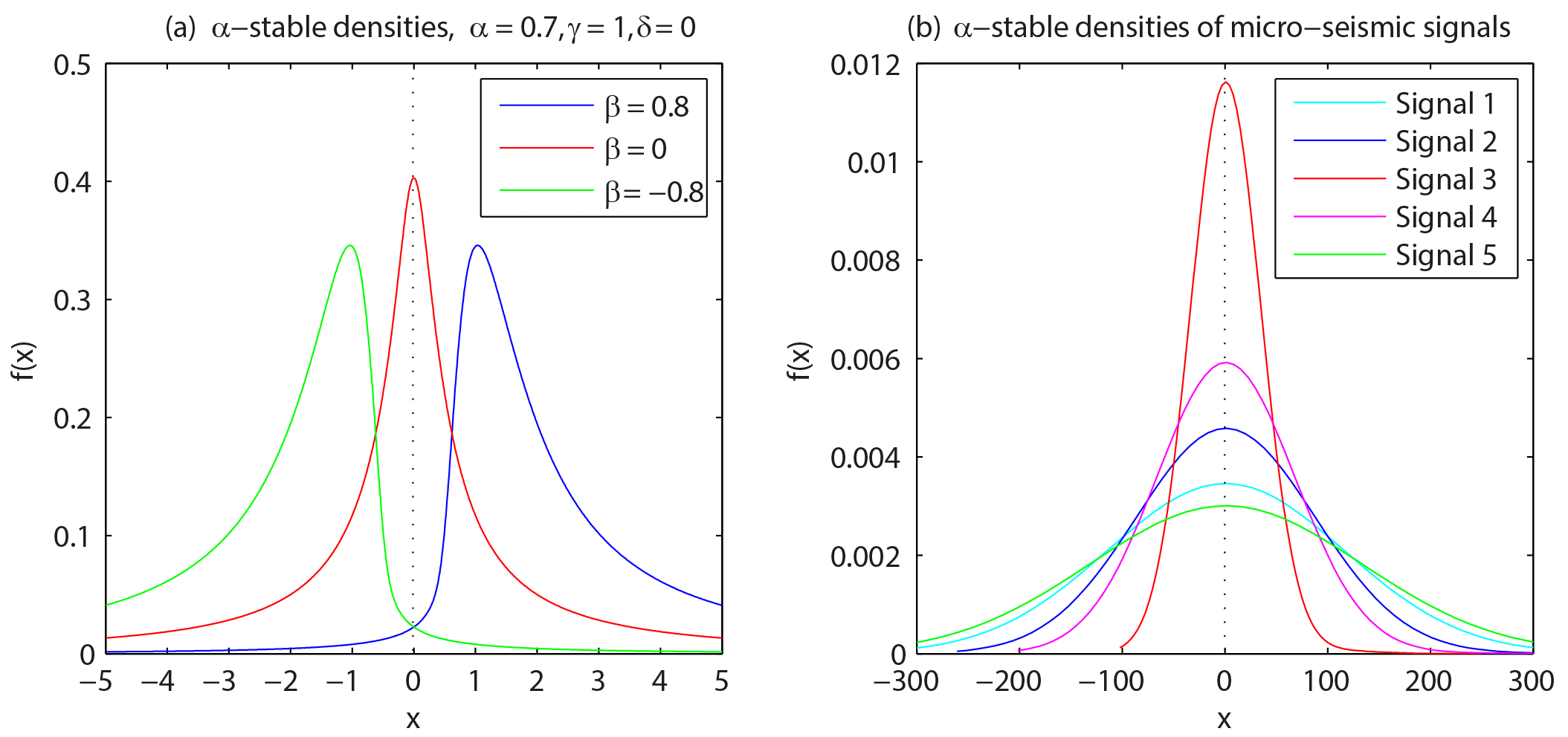
Figure 4(a) The α-stable densities with different skew parameter; (b) the α-stable densities of microseismic signals.
We select a measured microseismic wave and calculate its dynamic sample variance according to Eq. (10) (Fig. 3). It shows that the microseismic signal's dynamic sample variance jumps stepwise and also does not converge to a stable value. Thus, one can conclude that the microseismic signal follows the fractional lower-order α-stable distribution. Through the analysis of a large number of seismic signals and the calculation of characteristic exponents, current literature (Yue et al., 2013) shows that the characteristic exponent α of a seismic signal is less than 2, usually between 1.8458 and 1.9301.
2.4 The determination of symmetry property of microseismic signal
Before the parameter estimation of the α-stable distribution, we should determine whether the distribution of the signal is symmetric. The methods for identifying symmetry are listed below:
-
Draw the probability density curve of the sample sequence and observe the symmetry
-
Count the number of positive and negative values in the sample sequence. If the number of positive and negative values are approximately same, the signal is symmetric.
Figure 4a shows that when the skew parameter β=0, the probability density curve is symmetric; when β=0.8, the probability density curve is right-skewed; when , the probability density curve is left-skewed. Figure 4b shows five probability density curves of microseismic signals from the same seismic source. It is obvious that these curves are symmetric. As a result, the distribution of microseismic signal is considered symmetric.
For further validation of the symmetry of microseismic signal, we randomly select 30 signals from the microseismic records in different places, truncate the continuous 3000 sampling points of each signal and then count the number of positive and negative values. The absolute value for the difference between the numbers of positive and negative is shown in Fig. 5.
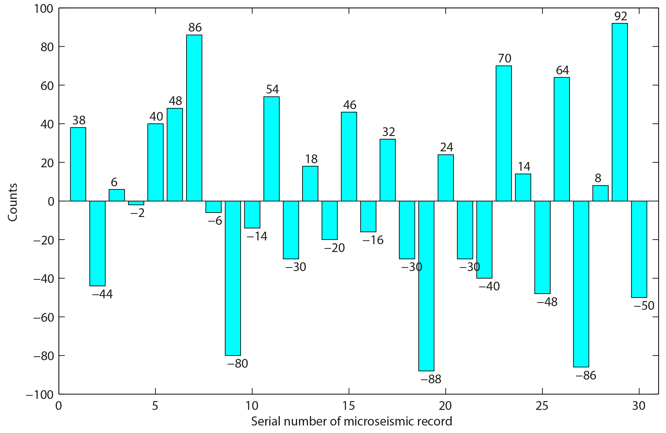
Figure 5The absolute value for the difference between the positive and negative counts in each microseismic record.
According to the data in Fig. 5, we can use estimate maximum likelihood estimator for parameters μ (difference of data number) and δ (standard error), and μ=1.8667 and δ=26.8356 are obtained. Compared with the 3000 of sample data, the microseismic signal is approximately considered symmetric.
In conclusion, the microseismic signal follows the symmetric α-stable distribution, which is also called the SαS distribution. Because the α-stable distribution does not have limited secondary and high-order moment, the above TDOA method is based on the assumption that the secondary moment (or high-order moment) and the Gaussian noise shows serious performance degradation. It is necessary to do some research on the new TDOA algorithm based on the low-order statistics.
3.1 The TDOA estimation based on FLOC
According to the study of Sect. 2.4, the microseismic signals and noises are more consistent with the α-stable distribution. Therefore, this paper is intended to describe the characteristics of microseismic signals and noises by α-stable distribution. ON this basis, an improved TDOA algorithm based on fractional low-order covariance (FLOC) is proposed. Compared with the traditional TDOA algorithm, the improved algorithm has a good suppression effect on the noise of α-stable distribution noise and Gauss noise.
In the case that the noise follows the α-stable distribution, an existing study (Ma and Nikias, 1995) puts forward a TDOA algorithm based on fractional low-order covariance (FLOC). The FLOC of two signals xi(t) () is defined as
and
where A and B represent the fractional low-order exponents of the two input signals xi(t) (), respectively. τ is the translation relative to the signal x1(t) when calculating FLOC. The TDOA estimation can be obtained by detecting the peak of the function Rd(τ).
The FLOC algorithm can be used for the TDOA estimation of microseismic signals. If the two microseismic signal samples are xi(n) (; , Eq. (12) can be expressed by
The TDOA estimation can be obtained by detecting the peak of the function.
The TDOA method based on FLOC requires very few calculations and its real-time implementation is simple. However, the α parameter needs to be estimated in advance; otherwise, the FLOC algorithm will have serious performance degradation and will lead to incorrect results when A and B are greater than α∕2.
3.2 The estimation of the characteristic exponent α
For the random variable X, which follows the α-stable distribution, the fractional lower-order moment is defined as E(|X|p), . p is the order of fractional lower-order moment. From the Zolotarev theorem (Zolotarev, 1966) we obtain
where α represents the characteristic exponent, γ represents the scale parameter and Γ(⋅) represents the gamma function.
If the random variable X follows the SαS distribution, a study has found that there is a negative-order moment in the SαS distribution (Ma and Nikias,1995). Equation (17) can then be changed to
because
Eq. (20) is continuous at the point p=0 after the introduction of negative-order moment. If Y=log |X|, E(epY) is the moment-generating function of Y and
Then any order moments of Y are limited and
This can be simplified to
where Ce=0.57721566… is a Euler constant. Then
For the microseismic signals Yi (, N is the sampling number), and the mean and variance can be obtained by Eqs. (25) and (26), respectively.
Plugging in the value gained from Eq. (26) into Eq. (24), we can obtain an estimated value of α. Then, the value of α is plugged into Eq. (23), and we obtain the value of γ.
3.3 Algorithm procedures
If xi(n) (; ) represents the sample of two microseismic signals from the same seismic source, the TDOA algorithm is shown below:
- Step 1:
-
for a given sequence of discrete signal x1(n) and x2(n), calculate their characteristic exponents α1 and α2 according to Eqs. (24), (25) and (26);
- Step 2:
-
assigning and to find that , , 0.95 is an empirical value;
- Step 3:
-
add the Hanning window to x1(n) and x2(n), and set the window lengths to max(size(x1(n))) and max(size(x2(n))). The cross-correlation function of x1(n) and x2(n) is calculated according to Eq. (15);
- Step 4:
-
detect the peak of the function . Then, the TDOA estimation can be obtained.
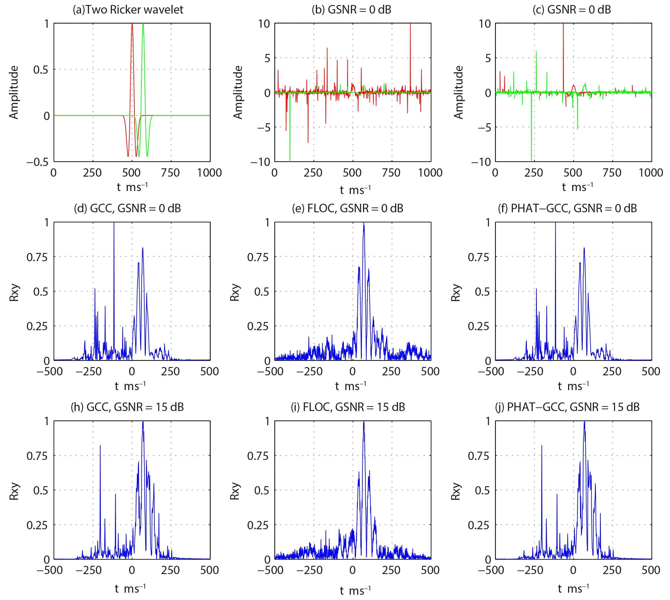
The signals Ricker1 and Ricker2 used in the simulation are two Ricker wavelets. Their spectral peak frequency is 25 Hz. The sampling frequency is 1 kHz, and the number of sampling points is 1000. The time delay between the two Ricker wavelets is set to 70 ms (Fig. 6a). The generalized signal-to-noise ratio (GSNR) is defined in Eq. (27) and used to describe the power ratio of signal and noise (Ma and Nikias, 1996).
In the equation, σs represents the signal power, and γ represents the noise figure of the α-stable distribution.
4.1 Experiment 1
The spatial resolution on TDOA estimation of the generalized cross correlation (GCC), PHAT-GCC (phase transfer–generalized correlation) method based on the Gaussian distribution and the FLOC method based on the non-Gaussian distribution are compared and verified. α-stable distribution noises to the two Ricker wavelets are added. The parameter of the α-stable distribution (α, β, γ, δ) is set to (1.2, 0, 1, 0). Because of the randomness of α-stable distribution noises, the two noises are independent of each other. The two Ricker wavelets with added noises are shown in Fig. 6b and c. In the case of α-stable distribution noises, the TDOA estimation results of the GCC, PHAT-GCC method and the FLOC method when GSNR = 0 dB and GSNR = 15 dB are shown in Fig. 6d–j.
It is evident from Fig. 6d, f, h and j that the GCC and PHAT-GCC method shows serious performance degradation when GSNR = 0 dB and GSNR = 15 dB. There are several peak positions in the curve so that the correct result is difficult to get. However, the FLOC method has a strong anti-interference ability. The peak appears at 70 ms and can estimate the time delay correctly.
4.2 Experiment 2
The influence of different α to the TDOA estimation results are verified. The two noises are generated randomly when α takes different values between 0 and 2 and are added to Ricker1 and Ricker2, respectively. When GSNR = 0 dB, the TDOA estimation result of the two signals with noises obtained by the FLOC method is shown in Fig. 7. Figure 7a–d show the waveforms of Ricker1 and Ricker2 with different noise signals added to these waveforms. Figure 7a*–d* show the corresponding TDOA estimation results.
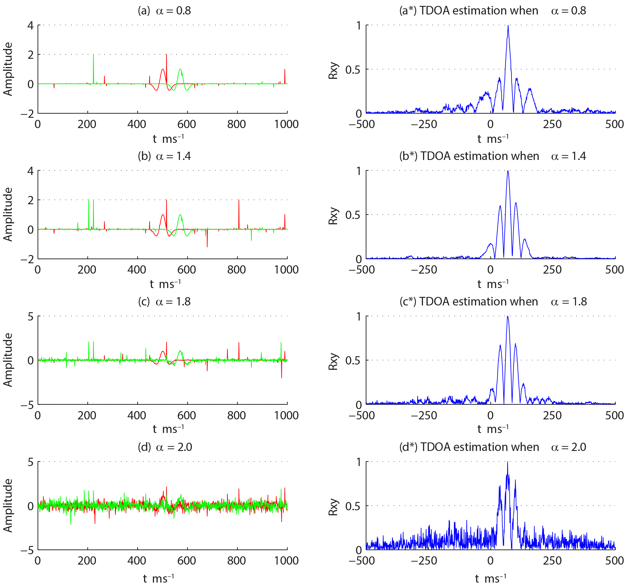
It is evident from Fig. 7 that a smaller α (which implies that there is a stronger pulse of noise) corresponds to better performance in the TDOA estimation of the FLOC algorithm. When α is close or equal to 2, the performance is degraded (Fig. 7d*), but it still can obtain the correct TDOA estimation result: 70 ms. Therefore, the FLOC method performs well irrespective of the noise and follows the Gaussian distribution or the α-stable distribution.
To verify the effectiveness of the FLOC method for TDOA estimation of real microseismic signals, we select eight microseismic signals from the same seismic source to do the experiment. The eight signals come from the ISS microseismic monitoring system of a coal mine in central China. Seismic geophones are laid along the mining roadway every 50 m in the system. The frequency bandwidth of the seismic geophones is between 3 and 2000 Hz. The data acquisition frequency is 1 kHz. For convenience of comparing and analyzing the experiment results, the first 2000 sampling points of each waveform are picked as the data object. The P arrival time of each microseismic signal is recorded manually, and the time delay between any two of the microseismic signals as a reference of the experimental result is calculated.
As an example, the microseismic signals in roadway nos. 2 and 7 are selected to explain the result. The waveforms of the microseismic signals after interception are shown in Fig. 8a and b. The time delay between the two signals obtained by manual method is 19 ms. First, when the microseismic signal follows the Gaussian distribution, the PHAT-GCC method, which, of the GCC methods, performs best, is chosen for the TDOA estimation of microseismic signals from the same seismic source. The result is shown in Fig. 8c. Second, when the microseismic signal follows the α-stable distribution, FLOC is used for the TDOA estimation. The characteristic exponent α of the two picked signals are calculated according to Eqs. (23), (24) and (25). α2=1.802, α7=1.835 are obtained as results. According to Step 2 in Sect. 3.3, assign A=0.85595 and B=0.87163. The TDOA estimation result obtained by the FLOC method is shown in Fig. 8d.
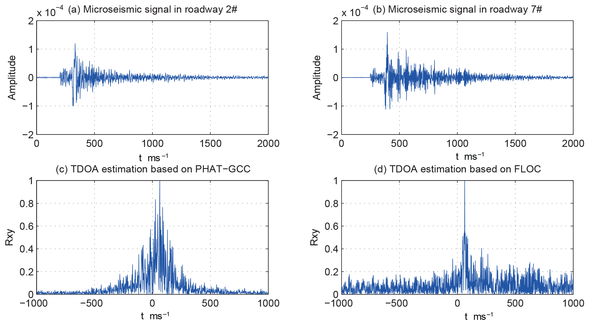
Figure 8c and d show that the two methods both obtain the correct result, 19 ms, but the peak of the FLOC method is sharper than the GCC method. This implies that the FLOC method performs better.
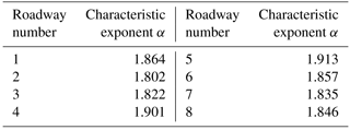
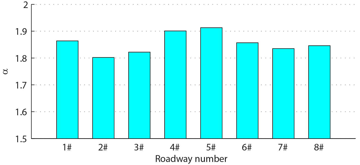
Each of the eight microseismic signals is considered to be a set of data following the α-stable distribution. Their characteristic exponent α values are calculated according to Eqs. (23), (24) and (25) and are shown in the table (Table 1). The values are between 1.802 and 1.913 (Fig. 9). It can be seen that the characteristic exponent α values of all of the signals are less than 2. According to the data in Table 1, we can use estimate maximum likelihood estimator for parameters μ (difference of data number) and δ (standard error), and μ=1.8550, δ=0.0377 can be obtained.
We can obtain 28 pairs of microseismic signals by the pair combination of the eight signals in Table 1. The comparison of TDOA estimations obtained by the PHAT-GCC, FLOC and manual method is shown in the table (Table 2).
Table 2The comparison of TDOA estimation results of microseismic signal.
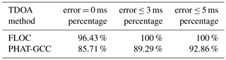
An analysis of tables (Tables 1, 2) indicates that the pulse of actual microseismic signal is stronger than the one following the Gaussian distribution. Because the characteristic exponent of the actual microseismic signal is less than 2, it is considered to be a signal following the α-stable distribution. Based on this observation, we can say that the spatial resolution of the FLOC method is better than the PHAT-GCC method at TDOA estimation of microseismic signals.
Through the analysis of the convergence of dynamic sample variance, the microseismic signal with noises is shown to follow the α-stable distribution. The analysis of the symmetry of probability density curve of the sample sequence proves that the microseismic signal is approximately symmetric. Therefore, it is more reasonable to regard the microseismic signal with noises as the α-stable distribution signal.
Because of the absence of second-order statistics of α-stable distribution, one cannot obtain optimal or correct estimation values via the traditional TDOA method based on the Gaussian distribution.
Microseismic monitoring data obtained from a coal mine in central China are used for TDOA estimation based on the GCC method and the FLOC method to study cases when the microseismic signals follow the Gaussian distribution and the α-stable distribution. In the comparison of the results and the time delay obtained manually, we observe that the FLOC method performs better than the traditional GCC method irrespective of whether the noise follows the Gaussian distribution or the α-stable distribution. This method is suitable for the TDOA estimation of microseismic signals from the same seismic source.
The microseismic data we use in this paper are derived from a coal mine. These microseismic data are not published online and are not intended to be published, because these data contain technical secrets of the coal mine.
The authors declare that they have no conflict of interest.
This work is funded by the State Key Research Development Program of China
(2016YFC0801406), the Key Research and Development Program of Shandong
Province (2017GSF20115), the Natural Science Foundation of Shandong Provice
(ZR2018MEE008), China Postdoctoral Science Foundation (2015M582117), Qingdao
Postdoctoral Applied Research Project and Special Project Fund of Taishan
Scholars of Shandong Province.
Edited by:
Shaun Lovejoy
Reviewed by: two anonymous referees
Carrier, A. and Got, J. L.: A maximum a posteriori probability time-delay estimation for seismic signals, Geophys. J. Int., 198, 1543–1553, 2014.
Choudhuri, S., Bharadwaj, S., Roy, N., Ghosh, A., and Ali, S. S.: Tapering the sky response for angular power spectrum estimation from low-frequency radio-interferometric data, Mon. Not. R. Astron. Soc., 459, 151–156, 2016.
Cornelis, B., Doclo, S., Tim, V. D. B., Moonen, M., and Wouters, J.: Theoretical analysis of binaural multi-microphone noise reduction techniques, IEEE T. Audio Speech, 18, 342–355, 2010.
Gedalyahu, K. and Eldar, Y. C.: Time-delay estimation from low-rate samples: a union of subspaces approach, IEEE T. Signal Proces., 58, 3017–3031, 2010.
Harada, K.: Nonparametric spectral estimation of phase noise in modulated signals based on complementary autocorrelation, IEEE T. Signal Proces., 62, 4479–4489, 2014.
He, X. L., She, T. L., and Gao, F.: A new method for picking up arrival times of seismic p and s waves automatically, Chinese J. Geophys.-Ch., 59, 2519–2527, 2016.
Hertz, D. and Azaria, M.: Time delay estimation between two phase shifted signals via generalized cross-correlation methods, Signal Process., 8, 235–257, 1985.
Hinich, M. J. and Wilson, G. R.: Time delay estimation using the cross bispectrum, IEEE T. Signal Proces., 40, 106–113 1992.
Hou, H., Sheng, G., Miao, P., Li, X., and Jiang, X.: Time-delay estimation algorithm of partial discharge UHF signals in substation based on bispectrum, Proceedings of the Chinese Society for Electrical Engineering, 33, 208–214, 2013 (in Chinese with English abstract).
Jia, R.-S., Zhao, T.-B., Sun, H.-M., and Yan, X.-H.: Microseismic signal denoising method based on empirical mode decomposition and Independent component analysis, Chinese J. Geophys.-Ch., 58, 1013–1023, https://doi.org/10.6038/cjg20150326, 2015.
Jia, R.-S., Liang, Y. Q., Hua, Y. C., Sun, H. M., and Xia, F. F.: Suppressing non-stationary random noise in microseismic data by using ensemble empirical mode decomposition and permutation entropy, J. Appl. Geophys., 133, 132–140, https://doi.org/10.1016/j.jappgeo.2016.08.001, 2016.
Jin, Z., Jiang, M., Sui, Q., Sai, Y., Lu, S., Cao, Y., Zhang, F., and Jia, L.: Acoustic emission localization technique based on generalized cross-correlation time difference estimation algorithm, Chinese J. Sensor. Actuat., 26, 1513–1518, 2013 (in Chinese with English abstract).
Kang, J. W., Whang, Y., Ko, B. H., and Kim, K. S.: Generalized cross-correlation properties of chu sequences, IEEE T. Inform. Theory, 58, 438–444, 2012.
Knapp, C. and Carter, G.: The generalized correlation method for estimation of time delay, IEEE T. Acoust. Speech, 24, 320–327, 1976.
Li, C. and Yu, G.: A new statistical model for rolling element bearing fault signals based on alpha-stable distribution, 2th International Conference on Computer Modeling and Simulation, Sanya China, 22–24 January 2010, 4, 386–390, 2010.
Ma, X. and Nikias, C. L.: Parameter estimation and blind channel identification in impulsive signal environments, IEEE T. Signal Proces., 43, 2884–2897, 1995.
Ma, X. and Nikias, C. L.: Joint estimation of time delay and frequency delay in impulsive noise using fractional lower order statistics, EEE T. Signal Proces., 44, 2669–2687, 1996.
Park, J., Shevlyakov, G., and Kim, K.: Maximin distributed detection in the presence of impulsive alpha-stable noise, IEEE T. Wirel. Commun., 10, 1687–1691, 2011.
Qiu, T. S., You, G. H., Sha, L., Zhao, X. P., and Gao, Y.: A phase spectrum time delay estimation method based on frequency difference compensation, Journal of Dalian University of Technology, 52, 90–94, 2012 (in Chinese with English abstract).
Salvati, D. and Canazza, S.: Adaptive time delay estimation using filter length constraints for source localization in reverberant acoustic environments, Signal Process. Lett., 20, 507–510, 2013.
Schwarz, B., Bauer, A., and Gajewski, D.: Passive seismic source localization via common reflection surface attributes, Stud. Geophys. Geod., 60, 531–546, 2016.
Shao, M. and Nikias, C. L.: Signal processing with fractional lower order moments: stable processes and their applications, P. IEEE, 81, 987–1010, 1993.
Souden, M., Benesty, J., and Affes, S.: Broadband source localization from an eigen analysis perspective, IEEE T. Audio Speech, 18, 1575–1587, 2010.
Sun, H. M., Jia, R. S., Du, Q. Q., and Fu, Y.: Cross-correlation analysis and time delay estimation of a homologous microseismic signal based on the Hilbert-Huang transform, Comput. Geosci., 91, 98–104, https://doi.org/10.1016/j.cageo.2016.03.012, 2016.
Sun, Y. M. and Qiu, T. S.: The new HB weighted time delay estimation algorithm under impulsive signal environments, J. Syst. Eng. Electron., 19, 1102–1108, 2008.
Wang, P., Zhang, X., Sun, G., Xu, L., and Xu, J.: Adaptive time delay estimation algorithm for indoor near-field electromagnetic ranging, Int. J. Commun. Syst., 30, e3113, https://doi.org/10.1002/dac.3113, 2017.
Xu, N., Dai, F., Sha, C., Lei, Y., and Li, B.: Microseismic signal characterization and numerical simulation of concrete beam subjected to three-point bending fracture, J. Sensors, 10, 1–11, 2015.
Youn, D. H., Ahmed, N., and Carter, G. C.: On using the LMS algorithm for time delay estimation, IEEE T. Acoust. Speech, 30, 798–801, 1982.
Yue, B., Peng, Z., and Zhang, Q.: Seismic inversion method with α-stable distribution, Chinese J. Geophys.-Ch., 55, 1307–1317, 2012 (in Chinese with English abstract).
Yue, B., Peng, Z., and Zhang, Q.: α-stable distribution seismic signal characteristic exponent estimation, Journal of Jilin University (Earth science edition), 43, 2026–2034, 2013 (in Chinese with English abstract).
Zhang, D. W., Bao, C. C., and Xia, B. Y.: Source localization based on time delay estimation in complex environment, J. Commun., 35, 183–190, 2014.
Zhang, S., Shen, G., An, L., and Niu, Y.: Online monitoring of the two-dimensional temperature field in a boiler furnace based on acoustic computed tomography, Appl. Therm. Eng., 75, 958–966, 2015.
Zhao, T. B., Guo, W. Y., Tan, Y. L., Lu, C. P., and Wang, C. W.: Case histories of rock bursts under complicated geological conditions, B. Eng. Geol. Environ., https://doi.org/10.1007/s10064-017-1014-7, online first, 2017.
Zolotarev, W. M.: On representation of stable laws by integrals, Selected Translations in Mathematical Statistics and Probability, 6, 84–88, 1966.