The adaptive particle swarm optimization technique for solving microseismic source location parameters

Sun, Hong-Mei; Yu, Jian-Zhi; Zhang, Xing-Li; Wang, Bin-Guo; Jia, Rui-Sheng

doi:https://doi.org/10.5194/npg-26-163-2019

Articles | Volume 26, issue 3

https://doi.org/10.5194/npg-26-163-2019

Articles | Volume 26, issue 3

Research article

15 Jul 2019

Research article |

| 15 Jul 2019

The adaptive particle swarm optimization technique for solving microseismic source location parameters

Hong-Mei Sun, Jian-Zhi Yu, Xing-Li Zhang, Bin-Guo Wang, and Rui-Sheng Jia

Abstract

An intelligent method is presented for locating a microseismic source based on the particle swarm optimization (PSO) concept. It eliminates microseismic source locating errors caused by the inaccurate velocity model of the earth medium. The method uses, as the target of PSO, a global minimum of the sum of squared discrepancies between differences of modeled arrival times and differences of measured arrival times. The discrepancies are calculated for all pairs of detectors of a seismic monitoring system. Then, the adaptive PSO algorithm is applied to locate the microseismic source and obtain optimal value of the P-wave velocity. The PSO algorithm adjusts inertia weight, accelerating constants, the maximum flight velocity of particles, and other parameters to avoid the PSO algorithm trapping by local optima during the solution process. The origin time of the microseismic event is estimated by minimizing the sum of squared discrepancies between the modeled arrival times and the measured arrival times. This sum is calculated using the obtained estimates of the microseismic source coordinates and P-wave velocity. The effectiveness of the PSO algorithm was verified through inversion of a theoretical model and two analyses of actual data from mine blasts in different locations. Compared with the classic least squares method (LSM), the PSO algorithm displays faster convergence and higher accuracy of microseismic source location. Moreover, there is no need to measure the microseismic wave velocity in advance: the PSO algorithm eliminates the adverse effects caused by error in the P-wave velocity when locating a microseismic source using traditional methods.

Download & links

Article (PDF, 351 KB)

How to cite

How to cite.

Dates

Received: 22 Mar 2019 – Discussion started: 02 Apr 2019 – Revised: 23 Jun 2019 – Accepted: 25 Jun 2019 – Published: 15 Jul 2019

1 Introduction

Microseismic monitoring technology can be used for effectively locating rock ruptures caused by rock burst, coal and gas outbursts, water inrush, and other coal mine disasters. In recent years it was also used in early warning systems (Li et al., 2016; Pastén et al., 2015; Jia et al., 2015). The spatial coordinates of monitoring stations and the arrival times of the first seismic wave are used to determine the coordinates of the microseismic source, origin time, and other attributes. The accuracy of microseismic source location has been an important research topic in microseismic monitoring technology for a long time.

Current microseismic source location methods mostly come from seismology. Now they are widely used in microseismic monitoring (Sun et al., 2016; Xue et al., 2015; Anikiev et al., 2014; Dong and Li, 2013). The earthquake source location method, based on time-difference principles, was proposed (Geiger, 1912). Based on this work, Lienert et al. (1986) developed an improved algorithm called HYPOCENTER. Since then, Nelson and Vidale (1990) presented the Quake3D method for 3-D velocity modeling. Lomax et al. (2000, 2001) worked out a nonlinear mode for locating global earthquakes in 3-D media and developed NonLinLoc software. Waldhauser and Ellsworth (2000) presented an earthquake location algorithm based on a double difference and developed HypoDD software. After occurrence of characteristics of the coal mine overburden, namely layers and abscission zones, Gong et al. (2012) proposed a microseismic detecting algorithm for the isotropic velocity model along the mine length; the algorithm decreases source location errors. Dong et al. (2017) proposed mathematical algorithms of microseismic source location where there is no need to predict velocity in advance. The algorithms overcome location errors caused by errors of velocity measurement inherent in traditional location methods. Lin et al. (2010) analyzed the characteristics of the linear location method and Geiger method and proposed a joint method to address the problem of low precision in estimation of source coordinates inherent in the linear location method. Feng et al. (2015) proposed stratified methods for microseismic source location based on particle swarm optimization to obtain correlations among the source position, origin time, and microseismic propagation speed for a non-unique solution.

In conclusion we note that the microseismic source location accuracy is influenced by many factors, such as the location method, the layout of the microseismic network, the velocity model, and the accuracy of the arrival-time measurement (Dong and Li, 2013). Among these, the key factor influencing the stability of the location algorithm and the location accuracy is precision of the velocity model (Prange et al., 2015; Li et al., 2014; Usher et al., 2013). In this paper, an adaptive particle swarm optimization algorithm is proposed for microseismic source location, which is based on average flying velocity of the particles. It uses, as the particle swarm optimization (PSO) target function, the least squares sum of measured arrival-time differences for all pairs of seismic sensors and uses the PSO algorithm to identify the source coordinates and microseismic wave velocity. Then, the origin time of the microseismic event is calculated according to the source location just determined and the wave velocity. Parameters of the PSO algorithm, such as the inertia weight, the acceleration constants, and the flight velocities of particles, are adaptively adjusted to avoid the algorithm failure caused by the improper selection of these parameters. Careful dynamic adjusting of the PSO parameters improves the robustness of the PSO algorithm, reduces the number of iterations, and improves estimation of the microseismic source coordinates and the seismic wave velocity.

2 Microseismic source location principle

Suppose that there are n geophones in the microseismic monitoring system. Set the microseismic source location point to $r_{0} = (x_{0}, y_{0}, z_{0})$ , the coordinates of each geophone to $r_{i} = (x_{i}, y_{i}, z_{i})$ and $(i = 1, \dots, n)$ , the time of P-wave arrival to the ith geophone of the microseismic monitoring system to t_i, and the origin time of the microseismic event to t₀. Assuming that the rock layers between the microseismic sources and the geophone are uniform (i.e., uniform velocity model), the equivalent average propagation velocity of the P wave in the medium is V. Then, the theoretical (regression) arrival-time differences for i and j geophones are

\begin{matrix} (1) & Δ t_{i, j} = t_{i} - t_{j} = \frac{l_{i} - l_{j}}{V}, i, j = (1, \dots, n), \end{matrix}

where

\{\begin{cases} l_{i} = \sqrt{{(x_{i} - x_{0})}^{2} + {(y_{i} - y_{0})}^{2} + {(z_{i} - z_{0})}^{2}} \\ l_{j} = \sqrt{{(x_{j} - x_{0})}^{2} + {(y_{j} - y_{0})}^{2} + {(z_{j} - z_{0})}^{2}} \end{cases} .

The differences between the difference of regression arrival times Δt_i,j(r₀) and the difference of the measured arrival times $Δ t_{i, j}^{'}$ are analogous to the double-difference concept introduced by Waldhauser and Ellsworth (2000). The sum of their squares reflect the degree of discrepancies between regression and observed arrival times. The equation for estimation of the microseismic source position has the form

\begin{matrix} (2) & Q (r_{0}, V) = \sum_{i, j = 1}^{n} {(Δ t_{i, j}^{'} - \frac{l_{i} (r_{0}) - l_{j} (r_{0})}{V})}^{2} = min_{r_{0}, V} . \end{matrix}

The estimates of microseismic source coordinates ${\hat{r}}_{0} = ({\hat{x}}_{0}, {\hat{y}}_{0}, {\hat{z}}_{0})$ and equivalent P-wave velocity in the medium $\hat{V}$ correspond to those values of $r_{0} = (x_{0}, y_{0}, z_{0})$ and V in Eq. (1) and Eq. (2), for which the function Q(r₀,V) reaches a global minimum in the ranges of possible values of the microseismic source coordinates and medium equivalent velocity.

According to time-difference location principles, the equation for calculation of the source origin time t₀ has the following form:

\begin{matrix} (3) & min_{t_{0}} F (t_{0}) = min_{t_{0}} \sum_{i = 1}^{n} {(t_{i}^{'} - t_{0} - \frac{l_{i} ({\hat{r}}_{0})}{\hat{V}})}^{2} . \end{matrix}

In the equation, $t_{i}^{'}$ denotes the measured travel times; for a case where signal-to-noise ratios in observed signals from microseismic source are sufficiently high and the earth medium between the source and geophones is homogeneous to $min_{r_{0}} F (t_{0}) \approx 0$ , the estimate of the microseism origin time can be calculated as

\begin{matrix} (4) & {\hat{t}}_{0} \approx \frac{1}{n} \sum_{i = 1}^{n} (t_{i}^{'} - \frac{l_{i} ({\hat{r}}_{0})}{\hat{V}}) . \end{matrix}

In solving for the seismic source location and origin time, the estimates of source coordinates ${\hat{r}}_{0} = ({\hat{x}}_{0}, {\hat{y}}_{0}, {\hat{z}}_{0})$ and the equivalent wave velocity $\hat{V}$ are obtained first, according to Eq. (2). Then, the estimate of the origin time is determined by substituting the estimated values ${\hat{r}}_{0}$ and $\hat{V}$ into Eq. (3) (or in Eq. 4 for the case where $min_{r_{0}} F (t_{0}) \approx 0)$ . Because Eq. (2) is a nonnegative function of (x₀, y₀, z₀) and V, a minimum $min_{r_{0}, V} Q (r_{0}, V)$ always exists and can be found by the nonlinear fitting methods. The classic method is the minimum least squares solution. However, in this solution the source location estimate ${\hat{r}}_{0}$ correlates with the origin-time estimate ${\hat{t}}_{0}$ , and the algorithm has a slow convergence for the velocity V. It is also easy to get a non-unique solution (Chen et al., 2009). To overcome these problems, this paper introduces an adaptive PSO algorithm to optimize the solution process.

Source location based on the time-difference principle is a multi-extremum nonlinear problem. The most popular method is the classical method proposed by Geiger (1912) and various improvements thereafter. This kind of method is a solution method in the linear category. According to Taylor's formula, the nonlinear problem is transformed into a linear problem, and then different strategies are adopted to solve the linear equation system. In many cases, such as those of a second order or more, this will appear. Problems such as in appropriate omitting of terms, unreasonable selection of initial values, and trapping solutions into local minima will occur (Lee and Stewart, 1981). The particle swarm optimization (PSO) method is simple to operate and easy to use, and it is easy to get the global optimal solution for multi-extremum nonlinear problems. Therefore, the improved PSO method is introduced to solve the above problems.

3 Adaptive PSO algorithm for solving location parameters

3.1 PSO principle

The PSO is an evolutionary computation technique developed by Eberhart and Kennedy (1995). It is an evolutionary algorithm similar to a simulated annealing optimization algorithm for a problem of iterative improvement of a candidate for the solution with regards to a given measure of quality. PSO is an intelligent computational algorithm for analyzing the dynamic behavior of a swarm of particles. In comparison with other similar algorithms, PSO has such advantages as simple implementation, high accuracy, and fast convergence. It has been successfully applied in the field of optimization in recent years (Fong et al., 2016; Renaudineau et al., 2015; Sudheeret al., 2014). The basic PSO principles are as follows: PSO randomly initializes a set of particles in the solution space. Each particle flies through the solution space with a certain speed by following the current optimum particle, and the optimal solution is found through the search in successive generations. In each generation, the particles update themselves by tracking two types of extreme values: local optimums and global optimums. The first extreme values are the optimal values for every particle itself in a set of positions of this particle in the sequence of generations that already exist. They are denoted as pBest. The second optimum is the optimal value found in the all existing generations of the whole swarm of particles. It is denoted as gBest. After the two sorts of the optimal values are found, the particles update their speed and positions according to Eq. (5):

\begin{matrix} (5) & \{\begin{cases} v_{i, d}^{(k + 1)} = w^{(k)} v_{i, d}^{(k)} + c_{1}^{(k)} r_{1} (p_{i, d}^{(k)} - x_{i, d}^{(k)}) + c_{2}^{(k)} r_{2} (p_{g, d}^{(k)} - x_{i, d}^{(k)}) \\ x_{i, d}^{(k + 1)} = x_{i, d}^{(k)} + v_{i, d}^{(k + 1)}, i = (1, \dots, n), d = (1, \dots, m) \end{cases}, \end{matrix}

where m is the dimension of the particle space, n is a number of particles in the swarm, k is a number of the current evolutionary particle generation, r₁ and r₂ are independent random values within [0, 1], w^(k) is the inertia weight at the kth particle generation, $c_{1}^{(k)}$ and $c_{2}^{(k)}$ are acceleration constants at the kth particle generation, $v_{i, d}^{(k)}$ is the current flight speed for the dth component of the ith particle at the kth generation, $x_{i, d}^{(k)}$ is the dth component of the ith particle's current location at the kth generation, $p_{i, d}^{(k)}$ is the dth coordinate of the current optimal value for the ith particle itself at the kth generation, and $p_{g, d}^{(k)}$ is the dth component of the current optimal value for the total particle population up to the kth generation.

3.2 The algorithm for solving source location parameters

Equation (2) concerns a nonlinear optimization problem with multiple local extrema. The PSO algorithm was developed for solving such problems and can be applied to search for the optimal value in four-dimensional solution space composed of (x, y, z, and v), that is, to solve for the source location and the equivalent seismic velocity. x, y, z, and v are the first, second, third, and fourth component of particles, respectively. The flow chart for the PSO algorithm is shown in Fig. 1.

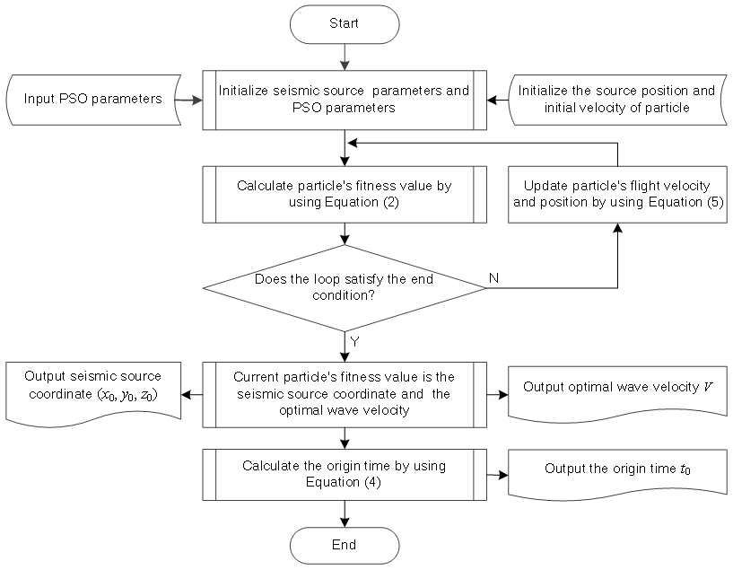
https://www.nonlin-processes-geophys.net/26/163/2019/npg-26-163-2019-f01

Figure 1Flow chart for the microseismic source location algorithm based on adaptive particle swarm optimization.

Download

The procedure for the source location parameter evaluation based on the PSO algorithm is described as follows.

Step 1. Initialize the model parameters for microseismic source location and the PSO parameters. Randomly initialize the source position and wave velocity of the PSO algorithm. Initialization of the PSO parameters mainly includes the population size m, acceleration constants c₁ and c₂, inertia weight w, computational accuracy ε, largest number of evolutionary generations T_max, initial velocity and positions of the particles, and maximum particle flight speed v_max. Then, initialize the iterative counter k.

Step 2. Calculate the particle (microseismic source coordinate and velocity model) fitness value by using Eq. (2). The calculated values here are the source's 3-D coordinates $(x_{0}^{(k)}, y_{0}^{(k)}, z_{0}^{(k)})$ and equivalent velocity V^(k), where k is the evolutionary generation number.

Step 3. Judge whether the current parameters of the particles meet the presupposed flight times and positioning accuracy or not. If they do, then go to Step 5; otherwise, go to Step 4.

Step 4. Update the flight velocity and particle positions according to Eq. (5), and then go back to Step 2.

Step 5. Output the estimated source's 3-D coordinates $({\hat{x}}_{0}, {\hat{y}}_{0}, {\hat{z}}_{0})$ and equivalent wave velocity $\hat{V} .$

Step 6. Calculate and output the origin-time estimate ${\hat{t}}_{0}$ by substituting estimated values of the source coordinates $({\hat{x}}_{0}, {\hat{y}}_{0}, {\hat{z}}_{0})$ and equivalent velocity $\hat{V}$ into Eq. (4). When the solution for the source coordinates and the origin time are obtained, the algorithm is over.

3.3 Discussion of PSO algorithm parameters

The parameter values for the PSO algorithm are the keys to influencing the algorithm performance and efficiency. This paper proposes guiding principles for adjusting parameters of the PSO algorithm based on the practical approach for solving for the seismic source parameters.

3.3.1 Inertia weight w^(k)

Generally, optimization problems are divided into local and global problems. The former consists of looking for the minimum in a finite area of function value space; the latter is for finding the minimum in the whole area of function value space. As early as 1998, Shi and Eberhart (1998) found that when the value of inertia weight w is relatively large, the global optimization ability of the PSO algorithm is strong, while the local optimization ability is weak. On the other hand, when the value of inertia weight w is relatively small, the local optimization ability of the PSO algorithm is strong, while the global optimization ability is weak. To avoid particles being stuck in a local optimum at the wrong time or missing the global optimal solution, this study uses the strategy of self-adaptive inertia weight to determine the proper value of w (Zhang and Liao, 2009). The strategy is the following.

In order to enhance the exploring competence of the PSO algorithm, the population average velocity should be maintained to be rather high at the initial stages of evolution, while in the late stage of evolution a smaller population average velocity should be maintained in order to strengthen the development capabilities of the algorithm. We assume that evolution of the average particle flying velocity with changing number of generations k should be close to the function defined by Eq. (6):

\begin{matrix} (6) & {\overline{v}}_{avg}^{(k)} = v_{e}^{(k)} = v_{0} e^{- {(\frac{2 k}{T_{\max} - T_{1}})}^{2}}, \end{matrix}

where v₀ represents the initial average velocity of population, T_max is the largest number of evolutionary generations, and T₁ is the number of evolved generations.

We will call $v_{e}^{(k)}$ the expected value of the average flying velocity for a particle population at the kth generation. The actual average velocity of the particle swarm at the kth generation is given by Eq. (7):

\begin{matrix} (7) & v_{avg}^{(k)} = \frac{1}{m} \sum_{i = 1}^{m} \sqrt{\sum_{d = 1}^{4} {(v_{i, d}^{(k)})}^{2}}, \end{matrix}

where $v_{i, d}^{(k)}$ represents the velocity of the dth component of the ith particle at the kth generation.

Set the initial inertia weight to w. Designate w^(k) inertia weight for the kth particle generation. Then the inertia weight w^(k+1) for the (k+l)th generation is determined by Eq. (8):

\begin{matrix} (8) & \{\begin{cases} if v_{avg}^{(k)} > v_{e}^{(k)} then w (k + 1) = w (k) / p \\ if v_{avg}^{(k)} < v_{e}^{(k)} then w (k + 1) = w (k) \cdot p \\ if v_{avg}^{(k)} = v_{e}^{(k)} then w (k + 1) = w (k) \\ if w (k + 1) > w_{max} then w (k + 1) = w_{max} \\ if w (k + 1) < w_{min} then w (k + 1) = w_{min} \end{cases}, \end{matrix}

where p is a some constant. Practice has proved that the best value of p is 1.05 (Zhang and Liao, 2009).

Substitution of w^(k) given by Eq. (8) into Eq. (5) ensures that average velocity $v_{avg}^{(k)}$ will reduce to zero in the process of population evolution.

3.3.2 Acceleration constants $c_{1}^{(k)}$ and $c_{2}^{(k)}$

Gao and Liao noted that the position $x_{i, d}^{(k)}$ of each particle in the population eventually converges to $(c_{1} p_{i, d} + c_{2} p_{g, d}) / (c_{1} + c_{2})$ (Gao and Liao, 2012). This means that the position of the particles for a large k will stay close to the lines that connect the global optimum point with the local optimum point. Therefore, in the first stage of particle swarm optimization, the optimum value of the particle itself is an important parameter for making all particles converge to global optimum.

However, if $c_{1}^{(k)}$ would be high for all k values, then the optimum position of the particle swarm would, generally, not coincide with the global optimum of the target function (2). Therefore, at the first stage of PSO, $c_{1}^{(k)}$ should take a larger value, while $c_{2}^{(k)}$ should take a smaller value to promote the local optimization speed. When particle swarm optimization is near its end, the role of the global optimal value should be highlighted. At this stage, $c_{1}^{(k)}$ should take a smaller value, while $c_{2}^{(k)}$ should take a larger value to help the particle swarm converge to the global optimum. Therefore, the acceleration constants $c_{1}^{(k)}$ and $c_{2}^{(k)}$ should be designed based on the average velocity of the particle swarm:

\begin{matrix} (9) & c_{1}^{(k)} = C \frac{v_{avg}^{(k)}}{v_{max}}, c_{2}^{(k)} = C (1 - \frac{v_{avg}^{(k)}}{v_{max}}) . \end{matrix}

C is a positive integer, usually in the range [2, 5].

3.3.3 The maximum flight velocity of particles v_max

The selection and analysis of the maximum flight velocity of particles should proceed as follows: if v_max is too small, then the particle movement will be restricted. In this situation, the algorithm cannot converge fast enough and may not even be able to achieve the optimal solution. On the other hand, if v_max is too large, then the optimal solution may be missed (Eslami et al., 2014; Abido, 2002). Therefore, it is very important to dynamically adjust the v_max value. To ensure uniform velocity through all dimensions, the maximum velocity in the dth dimension is proposed as

\begin{matrix} (10) & v_{max, d} = \frac{x_{max, d} - x_{min, d}}{N}, \end{matrix}

where x_max,d and x_min,d, respectively, stand for the largest and smallest values in the dth dimension of the possible particle positions, and N is a chosen number of intervals (Abido, 2002), usually in the range [1, 10].

4 Simulation and case study

4.1 Simulation analysis and discussion

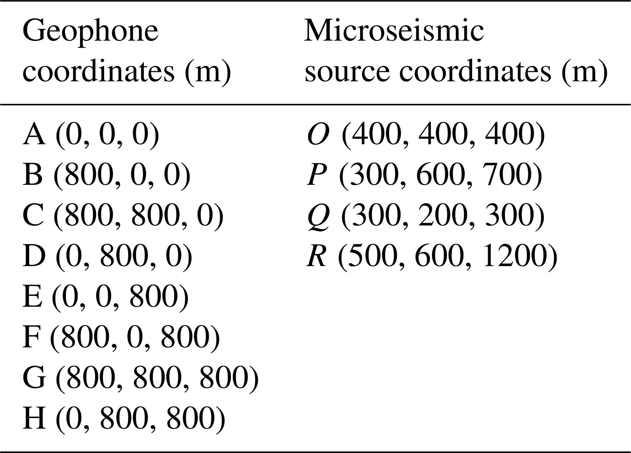
For the simulation, eight sensors comprising a microseismic localization system are located on the eight vertices of a cube. Four microseismic sources, O, P, and Q, are located inside the cube, and R is located outside of the cube. The coordinates of the geophones and the microseismic sources are shown in Table 1, and the relative locations of the geophones and microseismic sources are shown in Fig. 2.

Table 1Coordinates of sensors and microseismic sources.

Download Print Version | Download XLSX

https://www.nonlin-processes-geophys.net/26/163/2019/npg-26-163-2019-f02

Figure 2The locations of geophones and microseismic sources.

Download

It is assumed that the velocity of wave propagation (v) in the medium is unknown. According to the coordinates of geophones and microseismic sources shown in Table 1, first, the synthetic travel is computed. Then, the differences between the arrival times of all the pairs of the station are retrieved according to Eqs. (2), (3), and (4), and inversion is carried out by the least squares method (LSM; Dong et al., 2013) and the PSO proposed in this paper. The microseismic source location, equivalent wave velocity, and origin time are obtained. Then, the results calculated using the two different methods are compared using error analysis, the algorithm execution time, and the number of iterations.

Suppose a microseismic velocity of v=5.60 m ms⁻¹. According to the coordinate information in Table 1, the trigger time of the microseismic waves recorded by the geophones triggered can be calculated, as shown in Table 2. The method in this paper is PSO. The computational accuracy of the LSM algorithm is $ε = 1.0 \times 10^{- 10}$ . The parameters for the PSO algorithm are as follows: population size is m=50, w₀=1, and T_max=3000. The inertia weight w, acceleration constants c₁ and c₂, and maximum flight velocity of particles v_avg are determined by Eqs. (6)–(10). MATLAB programming was used to implement the LSM and PSO algorithms to obtain solutions at four points, O, P, Q, and R. The calculated results are shown in Table 3. The results of convergence are different when different initial values are selected for the LSM. When the initial value is far from the true value, the LSM satisfies the end condition, but it does not get the true value of the microseismic source. By repeatedly adjusting the initial value, the algorithm converges to the correct result. The corresponding initial values of the LSM in Table 3 are obtained after several adjustments. The PSO method can converge to the true value only by randomly selecting a set of initial values within a specified range.

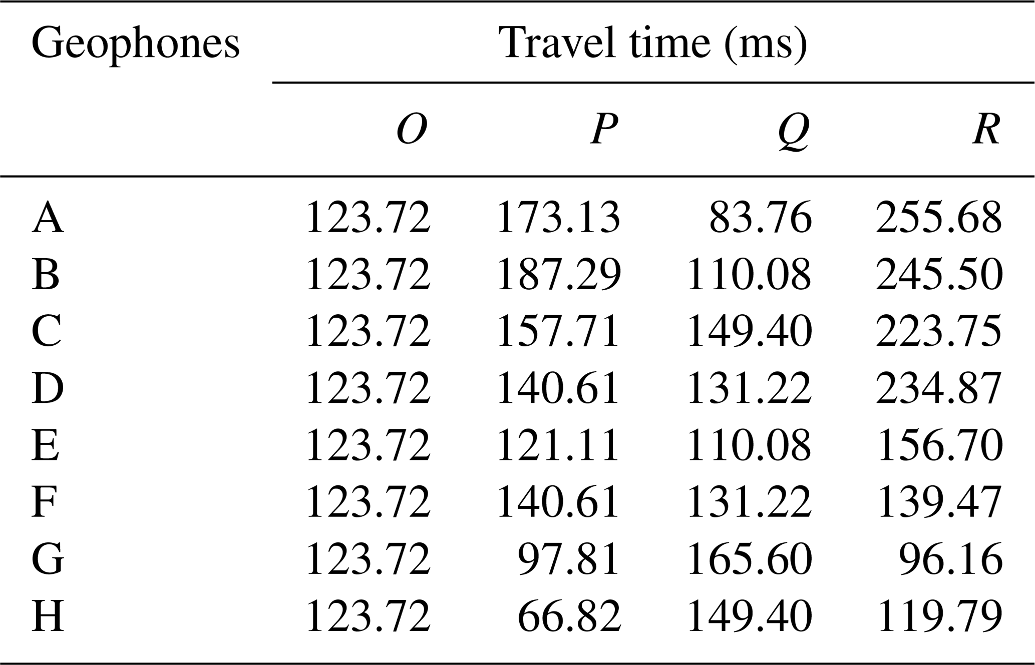
Table 2Travel time of a microseismic wave.

Download Print Version | Download XLSX

Table 3Comparison of the LSM and PSO algorithms.

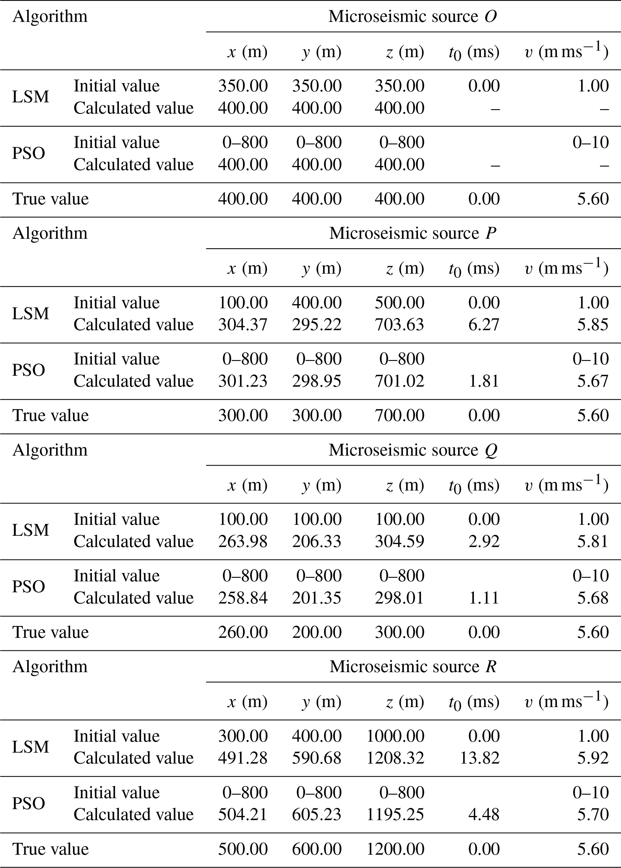
Note: “–” means that the value cannot be obtained directly. The calculated value from the PSO is the average value obtained after running the PSO algorithm 20 times.

Download Print Version | Download XLSX

Based on the results shown in Table 3, the LSM algorithm has different convergent results for different initial values. When the initial value is far from the true value, the required calculation accuracy ε can be met, but the result does not approach the true value. In some cases, there are multi-group results, so the initial values need to be repeatedly adjusted in order to make the LSM algorithm approach the true value. For the PSO algorithm, a wide range of initial values was used for the microseismic source location parameters. The only variables that need to be solved for are the 3-D coordinates of the arbitrary point inside the space surrounded by the seismic detection equipment. Thus, the calculated results can better approach the true value, and the solution is unique. This occurs because by improving the parameter selection rules, the condition where particles are trapped in local optima or fly over the global optimum during the process of searching is avoided; thus, the optimization ability of the PSO algorithm is improved.

Comparisons of the errors in the microseismic source location parameters obtained using the LSM and PSO algorithms are shown in Fig. 3, and the comparison of iterations between the two algorithms is shown in Fig. 4.

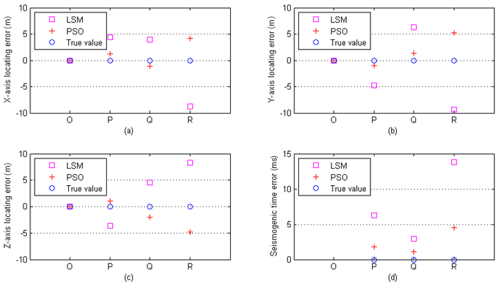
https://www.nonlin-processes-geophys.net/26/163/2019/npg-26-163-2019-f03

Figure 3Comparisons of the errors in the source location parameters between the LSM and PSO algorithms. (a) Comparisons of the x-axis locating error. (b) Comparisons of the y-axis locating error. (c) Comparisons of the z-axis locating error. (d) Comparisons of the errors in the origin-time estimation.

Download

https://www.nonlin-processes-geophys.net/26/163/2019/npg-26-163-2019-f04

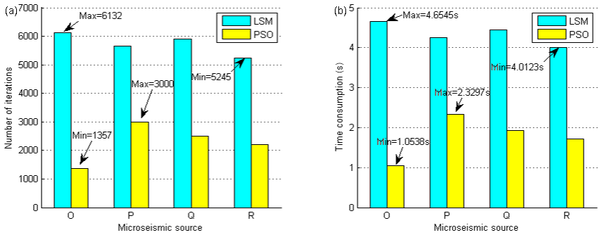
Figure 4(a) Comparison of the number of iterations between the LSM and PSO algorithms, where the max and min markers highlight the maximum and minimum number of iterations for each algorithm. (b) Comparison of the computing time between the LSM and PSO algorithms, where the max and min markers highlight the maximum and minimum amount of computing time for each algorithm.

Download

The selection of initial values for parameters in the LSM algorithm is comparatively complex, so the basic principle of parameter selection is to approach the desired value as near as possible. The selection of different initial values for parameters in the LSM algorithm has a greater influence on the accuracy of the solution location compared to PSO and results in a large difference in the number of iterations between the two methods. The improved PSO algorithm only needs to provide a value range for the initial parameters. Then, it automatically selects parameter values to iterate, and the algorithm runs for a maximum number of 3000 iterations. As is shown in Table 3, Fig. 3, and Fig. 4, compared with the LSM algorithm, the PSO algorithm not only improves the computational accuracy of the desired value of microseismic source parameters but also increases the computational efficiency and determines the microseismic source's real time location.

The following is a discussion of some special conditions. (1) Since source O is located at the cube's center of gravity, the distance between O and each geophone is the same. As a result, both the LSM and PSO algorithms can converge to the true value when solving for the seismic source coordinates (x₀, y₀, z₀) but cannot solve the origin time t₀ because regardless of which value of wave velocity v is selected, the value of Q in Eq. (2) tends to be zero. Because of the randomness of the wave velocity, the origin time t₀ cannot be solved according to Eq. (3). (2) Since source R is located outside of the cube, the average distance from this point to each sensor is larger than that from other points in the cube, such as P and Q points, to each sensor. The error in the equivalent wave velocity, which is solved by iteration, causes greater location error for R than for other points in the cube, so the layout of the seismic detection equipment should ensure that the microseismic source is within the detection array.

4.2 Case study

Because rock bursts occur frequently at a mine in central China, a Paladin 24-bit, multi-channel microseismic monitoring system of ESG Solutions in Canada was installed. In total, 18 seismic detection devices were installed in different positions at the mine: 9 seismic detection devices were installed at the −520 level, and 9 were installed at the −840 level. A blasting operation with a known position was conducted in order to verify the validity of the PSO algorithm. Ten seismic detection devices detected microseismic signals during the blasting operation. Pretreatments of the data, such as denoising and filtering, were performed on the detected signals in order to obtain a high SNR. Then, two blast points that showed an obvious rising waveform trend, making it easy to capture the trigger time, were selected and analyzed. The position coordinates of the two points are A (1495.60, 998.50, −685.10) and B (1298.70, 855.30, −576.20). The coordinates of the 10 seismic detection devices and the trigger times detected are shown in Table 4. The relative position of the 10 geophones and the two burst points is shown in Fig. 5. The seismic waveform data received by the geophone are shown in Fig. 6.

Table 4Geophone coordinates and travel time from the burst point.

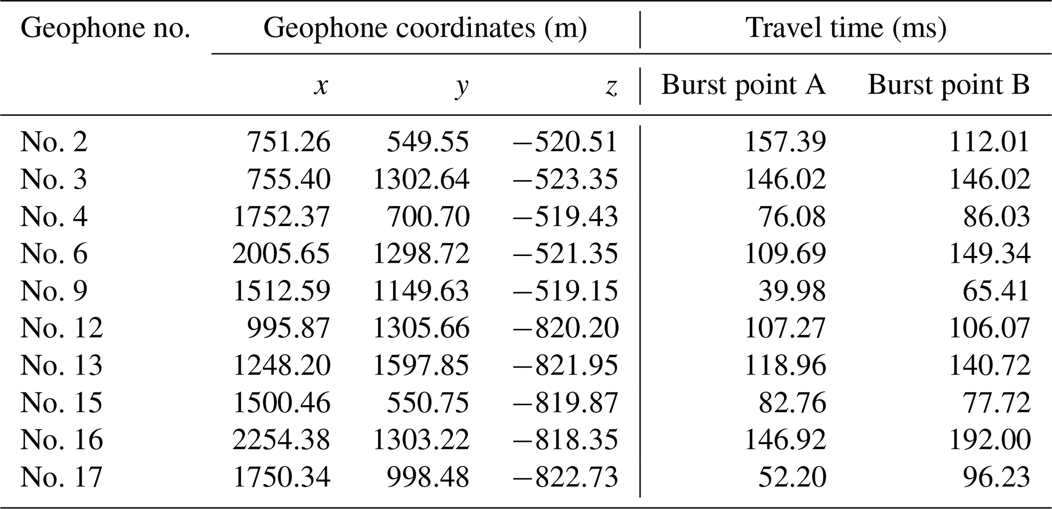
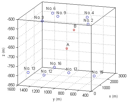
Download Print Version | Download XLSX

https://www.nonlin-processes-geophys.net/26/163/2019/npg-26-163-2019-f05

Figure 5Schematic diagram of the relative position of the 10 geophones and the two burst points.

Download

https://www.nonlin-processes-geophys.net/26/163/2019/npg-26-163-2019-f06

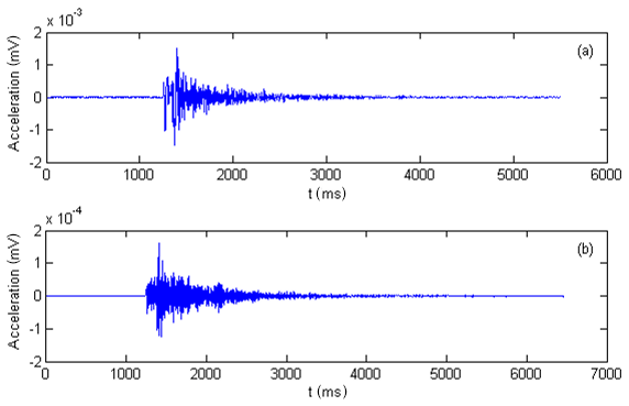
Figure 6(a) Seismic waveform of burst point A received by geophone no. 2. (b) Seismic waveform of burst point B received by geophone no. 2.

Download

The experiment was carried out on the advanced roadway of the coal mine working face. The diameter of the borehole is 42 mm, the depth of the borehole is 1.2 m, and the length of the filled explosive is one-fourth of the borehole depth. We approximate the blasting point to a spherical blasting point without considering the error caused by the assumption. Based on the data presented in Table 4, the PSO algorithm and LSM algorithm were used to solve for the seismic source location parameters and origin time. A comparison of the error is shown in Table 5.

Table 5Error comparison for the LSM algorithm and PSO algorithm.

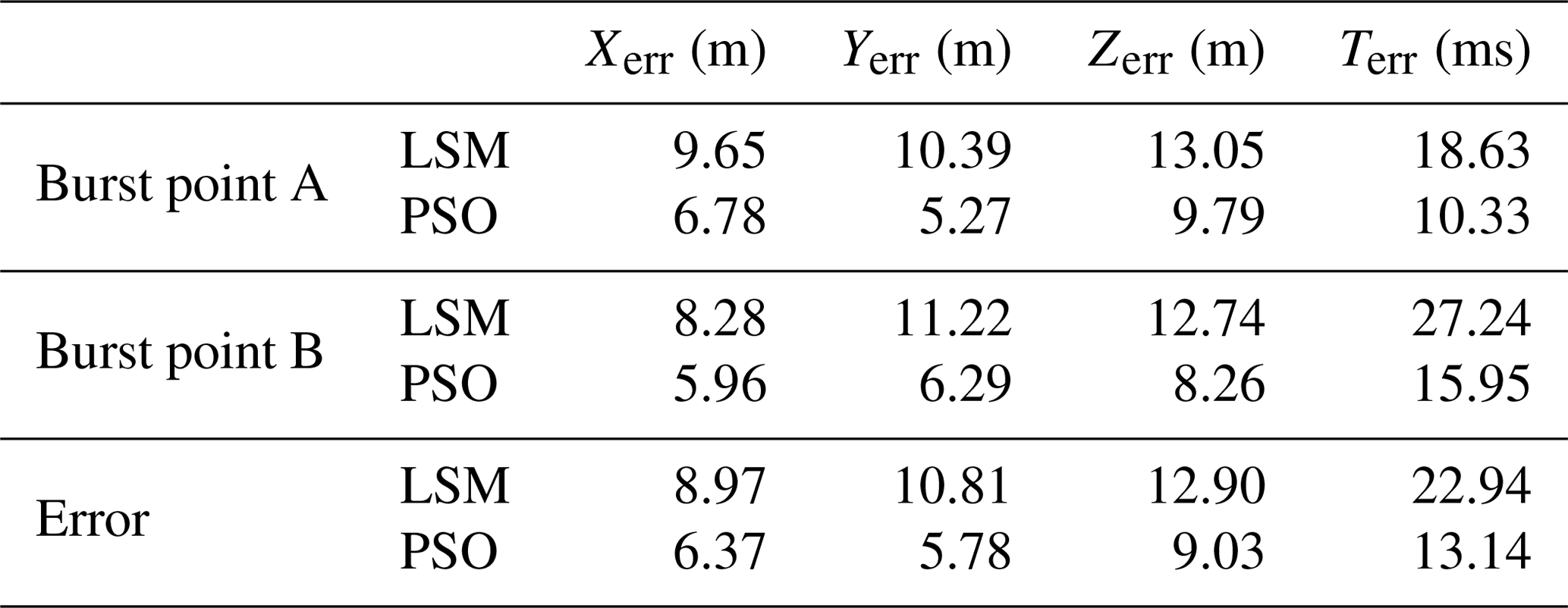
Download Print Version | Download XLSX

According to Table 5, the accuracy of the LSM algorithm is relatively poor. Its average deviation in the X, Y, and Z directions is 8.97, 10.81, and 12.90 m, respectively. The results were obtained after repeated adjustment of the initial location parameters for the seismic source and the wave velocity. The PSO algorithm can automatically approach the true values according to the given initial parameter range. Its average deviation in the X, Y, and Z directions is 6.37, 5.78, and 9.03 m, respectively, with errors that are less than 5 %. Therefore, the PSO can achieve high positioning accuracy in the geophone range.

The simulation example and blasting experiment discussed above clearly demonstrate that the PSO optimization algorithm is better than the LSM when solving for the microseismic positioning parameters and the seismic origin time. The algorithm has high positioning accuracy and fast convergence speed, and it is easy to set the initial parameters. This is because the adaptive PSO algorithm is more accurate in fitting the relationship between each coordinate for the seismic detection equipment and the time difference. It can dynamically adjust the velocity value in an iterative process until the value approximates the optimal average velocity, which can account for the nonlinear relationship between each coordinate of the seismic detection equipment and the time difference and can greatly reduce the impact of the velocity error on the positioning precision.

4.3 Discussion

In order to further verify the effectiveness of the proposed method, the experiments in Sect. 4.1 are compared and analyzed under different wave velocities. The comparative analysis steps are as follows. (1) Use the PSO method and the LSM to locate the microseismic source when using real velocity (i.e., error floating at 0 %). (2) Because it is difficult to measure real wave velocity in practical engineering, small errors of 1 %, 3 %, and 5 % are given to the PSO method and LSM; in other words, when the wave velocity is 5.544, 5.432, and 5.320 m ms⁻¹, two methods are used to locate the microseismic source. (3) Step 1 and Step 2 are used to locate the microseismic source, and the absolute distance error is calculated by comparing the locating results with the real values. The absolute distance errors calculated by the PSO method and the LSM at different wave velocities are plotted in Fig. 7.

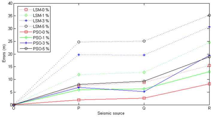
https://www.nonlin-processes-geophys.net/26/163/2019/npg-26-163-2019-f07

Figure 7Comparison of locating errors between PSO method and LSM at different wave velocities.

Download

As we can be seen from Fig. 7, the LSM will cause large errors in the location system under the disturbance of different wave velocities. The maximum error is up to 25 m (except for the seismic source R), while the PSO method is more stable. The reason is that the PSO method can accurately fit the relationship between the coordinates of each sensor and the time difference because it does not depend on the velocity value when solving the seismic location parameters. The LSM needs accurate velocity to solve the seismic location parameters, and the disturbance of velocity has a great influence on the results. That is to say, in the case of wave velocity disturbance, even if there is a small error in the value of wave velocity, there will be a large error in the location result of the LSM. Because of the complexity of rock media, the average velocity of each region is not necessarily the same, and due to the influence of construction technology, it is very difficult to determine the velocity of anisotropic media; this is the main reason for the low positioning accuracy of the LSM. In addition, when the source is outside of the sensor array (such as seismic source R), the errors of the two methods are very large, but the LSM has greater locating errors than the PSO method, which shows that the sensor arrangement should ensure that the seismic source is within the array as far as possible.

5 Conclusions

An adaptive PSO optimization method is proposed based on the average population velocity in order to solve for location parameters of the seismic source in a location model. This method takes the minimum residual sum of squares between the time-difference regression values and the time-difference measured values for two seismic detection devices, and the PSO algorithm is designed to solve for the seismic source coordinates and the equivalent wave velocity and then solve for the seismic source origin time.
Combined with the actual need to solve for seismic source parameters, the model constraints of inertia weight, accelerating constants, the maximum flight velocity of particles, and other parameters are discussed in order to improve the optimization capacity of the PSO algorithm and avoid being trapped in a local optimum.
Comparative analysis shows that when solving for the seismic source location parameters, compared with the classic least squares method, the adaptive PSO algorithm has high positioning accuracy and fast convergence, and it is easy to set the initial parameter values.

Data availability

Data and results of calculations are available by e-mail request.

Author contributions

HMS designed the study, performed the research, analyzed data, and wrote the paper. JZY performed the analysis with constructive discussions. XLZ helped performed the data analyzes. BGW contributed to the collection and analysis of the data. RSJ contributed to refining the ideas, carrying out additional analyses, and finalizing this paper.

Competing interests

The authors declare that they have no conflict of interest.

Acknowledgements

The authors wish to thank the two anonymous reviewers and editor for their suggestions for improving the paper. They are also grateful for collaborative funding support from the Key Research and Development Program of Shandong Province (grant nos. 2017GSF20115 and 2018GGX109013), the Natural Science Foundation of Shandong Province (grant no. ZR2018MEE008), and the project of the Shandong Province High Educational Science and Technology Program (grant no. J18KA307).

Financial support

This research has been supported by the Key Research and Development Program of Shandong Province (grant nos. 2017GSF20115 and 2018GGX109013), the Natural Science Foundation of Shandong Province (grant no. ZR2018MEE008), and the project of the Shandong Province High Educational Science and Technology Program (grant no. J18KA307).

Review statement

This paper was edited by Luciano Telesca and reviewed by two anonymous referees.

References

Abido, M. A.: Optimal power flow using particle swarm optimization, Int. J. Electr. Power Energy Syst., 24, 563–571, 2002.

Anikiev, D., Valenta, J., Staněk, F., and Eisner, L.: Joint location and source mechanism inversion of microseismic events: benchmarking on seismicity induced by hydraulic fracturing, Geophys. J. Int., 198, 249–258, 2014.

Chen, B., Feng, X., Li, S., Yuan, J., and Xu, S.: Microseism source location with hierarchical strategy based on particle swarm optimization, Chin. J. Rock Mech. Eng., 28, 740–749, 2009.

Dong, L. and Li, X.: A microseismic/acoustic emission source location method using arrival times of ps waves for unknown velocity system, Int. J. Distrib. Sens. Netw., 2013, 485–503, 2013.

Dong, L., Sun, D., Li, X., and Du, K.: Theoretical and experimental studies of localization methodology for ae and microseismic sources without pre-measured wave velocity in mines, IEEE Access, 99, 16818–16828, 2017.

Eberhart, R. C. and Kennedy, J.: A new optimizer using particle swarm theory, Proceedings of the Sixth International Symposium on Micro Machine and Human Science, 4–6 October, Nagora, Japan, 39–43, 1995.

Eslami, M., Shareef, H., Taha, M. R., and Khajehzadeh, M.: Adaptive particle swarm optimization for simultaneous design of upfc damping controllers, Int. J. Electr. Power Energy Syst., 57, 116–128, 2014.

Feng, G. L., Feng, X. T., Chen, B. R., Xiao, Y. X., and Jiang, Q.: Sectional velocity model for microseismic source location in tunnels, Tunn. Undergr. Sp. Tech., 45, 73–83, 2015.

Fong S., Wong R., and Vasilakos A.: Accelerated PSO swarm search feature selection for data stream mining big data, IEEE Trans. Serv. Comput., 9, 33–45, 2016.

Gao, Z. and Liao, X. Z.: Hybrid adaptive particle swarm optimization based on average velocity, Control Decis., 27, 376–381, 2012.

Geiger, L.: Probability method for the determination of earthquake epicenters from arrival time only, Bull. St. Louis. Univ., 8, 60–71, 1912.

Gong, S. Y., Dou, L. M., Ma, X. P., Mou, Z. L., He, H., and He, J.: Study on the construction and solution technique of anisotropic velocity model in the location of coal mine tremor, Chinese J. Geophys.-Chinese Ed., 55, 1757–1763, 2012.

Lee, W. H. K. and Stewart, S. W.: Principles and applications of microearthquake networks, Academic Press, New York, 1981.

Jia, R. S., Liu, C., Sun, H. M., and Yan, X. H.: A situation assessment method for rock burst based on multi-agent information fusion, Comput. Electr. Eng., 45, 22–32, 2015.

Li, N., Wang, E., Ge, M., and Sun, Z.: A nonlinear microseismic source location method based on simplex method and its residual analysis, Arab. J. Geosci., 7, 4477–4486, 2014.

Li, X., Wang, E., Li, Z., Liu, Z., Song, D., and Qiu, L.: Rock burst monitoring by integrated microseismic and electromagnetic radiation methods, Rock Mech. Rock Eng., 49, 1–14, 2016.

Lienert, B. R., Berge, E., and Frazer, L. N.: Hypocenter: an earthquake location method using centered, scaled, and adaptively damped least squares, Bull. Seismol. Soc. Amer., 6, 771–783, 1986.

Lin, F., Li, S. L., Xue, Y. L., and Xu, H. B.: Microseismic sources location methods based on different initial values, Chin. J. Rock Mech. Eng., 29, 996–1002, 2010.

Lomax, A., Virieux, J., Volant, P. and Berge, C.: Probabilistic earthquake location in 3-D and layered models: Introduction of a Metropolis-Gibbs method and comparison with linear locations, in: Advances in Seismic Event Location, edited by: Thurber, C. H. and Rabinowitz, N., Kluwer, Amsterdam, 101–134, 2000.

Lomax, A., Zollo, A., Capuano, P., and Virieux, J.: Precise, absolute earthquake location under Somma-Vesuvius volcano using a new 3-D velocity model, Geophys. J. Int., 146, 313–331, 2001.

Nelson, G. D. and Vidale, J. E.: Earthquake locations by 3-D finite difference travel times, Bull. Seismol. Soc. Amer., 80, 395–410, 1990.

Pastén, D., Estay, R., Comte, D., and Vallejos, J.: Multifractal analysis in mining microseismicity and its application to seismic hazard in mine, Int. J. Rock Mech. Min. Sci., 78, 74–78, 2015.

Prange, M. D., Bose, S., Kodio, O., and Djikpesse, H. A.: An information-theoretic approach to microseismic source location, Geophys. J. Int., 201, 193–206, 2015.

Renaudineau, H., Donatantonio, F., Fontchastagner, J., Petrone, G., Spagnuolo, G., Martin, J., and Pierfederici, S.: A PSO-based global mppt technique for distributed PV power generation, IEEE Trans. Ind. Electron., 62, 1047–1058, 2015.

Shi, Y. and Eberhart, R. C.: Parameter selection in particle swarm optimization, Evolutionary Programming VII, Springer, Berlin Heidelberg, 1998.

Sudheer, C., Maheswaran, R., Panigrahi, B. K., and Marthur, S.: A hybrid SVM-PSO model for forecasting monthly streamflow, Neural Comput. Appl., 24, 1381–1389, 2014.

Sun, H. M., Jia, R. S., Du, Q. Q., and Fu, Y.: Cross-correlation analysis and time delay estimation of a homologous micro-seismic signal based on the Hilbert-Huang transform, Comput. Geosci., 91, 98–104, 2016.

Usher, P. J., Angus, D. A., and Verdon, J. P.: Influence of a velocity model and source frequency on microseismic waveforms: some implications for microseismic locations, Geophys. Prospect., 61, 334–345, 2013.

Waldhauser, F. and Ellsworth, W. L.: A double-difference earthquake location algorithm: method and application to the northern Hayward fault, California, Bull. Seismol. Soc. Amer., 90, 1353–1368, 2000.

Xue, Q., Wang, Y., Zhan, Y., and Chang, X.: An efficient gpu implementation for locating micro-seismic sources using 3d elastic wave time-reversal imaging, Comput. Geosci., 82, 89–97, 2015.

Zhang, D. X. and Liao, R. Q.: Adaptive particle swarm optimization algorithm based on population velocity, Control Decis., 24, 1257–1246, 2009.

Articles

Short summary

An adaptive PSO optimization method is proposed based on the average population velocity in order to solve for location parameters of the seismic source in a location model. Combined with the actual need to solve for seismic source parameters, the model constraints of inertia weight, accelerating constants, the maximum flight velocity of particles, and other parameters are discussed in order to improve the optimization capacity of the PSO algorithm and avoid being trapped in a local optimum.

The adaptive particle swarm optimization technique for solving microseismic source location parameters

3.1 PSO principle

3.2 The algorithm for solving source location parameters

3.3 Discussion of PSO algorithm parameters

3.3.1 Inertia weight w(k)

3.3.2 Acceleration constants c1k and c2k

3.3.3 The maximum flight velocity of particles vmax

4.1 Simulation analysis and discussion

4.2 Case study

4.3 Discussion

3.3.1 Inertia weight w^(k)

3.3.2 Acceleration constants $c_{1}^{(k)}$ and $c_{2}^{(k)}$

3.3.3 The maximum flight velocity of particles v_max