the Creative Commons Attribution 4.0 License.
the Creative Commons Attribution 4.0 License.
 | 24 Jul 2019
Data assimilation using adaptive, non-conservative, moving mesh models
Alberto Carrassi
Colin T. Guider
Chris K. R. T Jones
Pierre Rampal
Numerical models solved on adaptive moving meshes have become increasingly prevalent in recent years. Motivating problems include the study of fluids in a Lagrangian frame and the presence of highly localized structures such as shock waves or interfaces. In the former case, Lagrangian solvers move the nodes of the mesh with the dynamical flow; in the latter, mesh resolution is increased in the proximity of the localized structure. Mesh adaptation can include remeshing, a procedure that adds or removes mesh nodes according to specific rules reflecting constraints in the numerical solver. In this case, the number of mesh nodes will change during the integration and, as a result, the dimension of the model's state vector will not be conserved. This work presents a novel approach to the formulation of ensemble data assimilation (DA) for models with this underlying computational structure. The challenge lies in the fact that remeshing entails a different state space dimension across members of the ensemble, thus impeding the usual computation of consistent ensemble-based statistics. Our methodology adds one forward and one backward mapping step before and after the ensemble Kalman filter (EnKF) analysis, respectively. This mapping takes all the ensemble members onto a fixed, uniform reference mesh where the EnKF analysis can be performed. We consider a high-resolution (HR) and a low-resolution (LR) fixed uniform reference mesh, whose resolutions are determined by the remeshing tolerances. This way the reference meshes embed the model numerical constraints and are also upper and lower uniform meshes bounding the resolutions of the individual ensemble meshes. Numerical experiments are carried out using 1-D prototypical models: Burgers and Kuramoto–Sivashinsky equations and both Eulerian and Lagrangian synthetic observations. While the HR strategy generally outperforms that of LR, their skill difference can be reduced substantially by an optimal tuning of the data assimilation parameters. The LR case is appealing in high dimensions because of its lower computational burden. Lagrangian observations are shown to be very effective in that fewer of them are able to keep the analysis error at a level comparable to the more numerous observers for the Eulerian case. This study is motivated by the development of suitable EnKF strategies for 2-D models of the sea ice that are numerically solved on a Lagrangian mesh with remeshing.


1.1 Adaptive mesh models
The computational model of a physical phenomenon is typically based on solving a particular partial differential equation (PDE) with a numerical scheme. Numerical techniques to solve PDEs evolving in time are most often based on a discretization of the underlying spatial domain. The resulting mesh is generally fixed in time, but the needs of a given application may require the mesh itself to change as the system evolves, adapting to the underlying physics (Weller et al., 2010). We consider here the impact of such a numerical approach on data assimilation.
Two reasons that may lead to the use of an adaptive mesh are as follows: (1) for fluid problems, it is sometimes preferable to pose the underlying PDEs in a Lagrangian, as opposed to Eulerian, frame or (2) the model produces a specific structure, such as a front, shock wave or overflow, which is localized in space. In case 1, the Lagrangian solver will naturally move the mesh with the evolution of the PDE (Baines et al., 2011). For case 2, the idea is to improve computational accuracy by increasing the mesh resolution in a neighborhood of the localized structure (see, e.g., Berger and Oliger, 1984). This may be compensated by the decrease in resolution elsewhere in the domain. Adapting the mesh can prove computationally efficient in that an adaptive mesh generally requires fewer points than a fixed mesh to attain the same level of accuracy (Huang and Russell, 2010). Some important application areas where adaptive meshes have been used are groundwater equations (Huang et al., 2002) and thin film equations (Alharbi and Naire, 2017) as well as large geophysical systems (Pain et al., 2005; Davies et al., 2011).
1.2 Data assimilation for adaptive mesh models: the issue
Data assimilation (DA) is the process by which data from observations are assimilated into a computational model of a physical system. There are numerous mathematical approaches, and associated numerical techniques, for approaching this issue (see, e.g., Budhiraja et al., 2018). We use the term DA to refer to the collection of methods designed to obtain an estimate of the state and parameters of the system of interest using noisy, usually unevenly distributed data and an inevitably approximate model of its evolution (see, e.g., Asch et al., 2016). There has been considerable development of DA methods in the field of the geosciences, particularly as a tool to estimate accurate initial conditions for numerical weather prediction models; a review on the state-of-the-art DA for the geosciences can be found in Carrassi et al. (2018).
Mesh adaptation brings significant challenges to DA. In particular, a time-varying mesh may introduce difficulties in the gradient calculation within variational DA (Fang et al., 2006). In an ensemble DA methodology (Evensen, 2009; Houtekamer and Zhang, 2016), the challenge arises from the need to compare different ensemble members in the analysis step. With a moving mesh that depends on the initialization, different ensemble members may be made up of physical quantities evaluated at a different set of spatial points. There is another variation that is key to our considerations here and that is relevant in both cases described above. The issue is that the nodes in the mesh may become too close together or too far apart. Both situations can lead to problems with the computational solver. Some adjustment of the mesh, based on some prescribed tolerance, may then be preferable and even necessary. We are particularly interested in the implications for DA when this adjustment involves the insertion or deletion of nodes in the mesh. The size of the mesh may then change in time, which has the consequence that the state vectors at different times may not have the same dimension. In other words, the state space itself is changing in dimension with time. Consequently, individual ensemble members, each of them representing a possible realization of the state vector, can even have different dimensions. In this situation, it is not possible to straightforwardly compute the ensemble-based error mean and error covariances that are necessary and are at the core of the ensemble DA methods (Evensen, 2009). Dealing with and overcoming this situation is the main aim of this study.
Two specific pieces of work can be viewed as precursors of our methodology. Bonan et al. (2017) study an ice sheet that is moving and modeled by a Lagrangian evolution but without remeshing. The paper by Du et al. (2016) develops DA on an unstructured adaptive mesh. Their mesh is adapted to the underlying solution to better capture localized structures with a procedure that is akin to the remeshing in neXtSIM. The challenge we address here is the development of a method that will address models that are based on Lagrangian solvers and involve remeshing.
1.3 Motivation: the Lagrangian sea-ice model neXtSIM
This work is further motivated by a specific application, namely performing ensemble-based DA for a new class of computational models of sea ice (Bouillon et al., 2018). In particular, the setup we develop is based on the specifications of neXtSIM, which is a stand-alone finite element model employing a Maxwell elasto-brittle rheology (Dansereau et al., 2016; Rampal et al., 2019) to simulate the mechanical behavior of the sea ice. In this new rheological framework, the heterogeneous and intermittent character of sea-ice deformation (Marsan et al., 2004; Rampal et al., 2008) is simulated via a combination of the concepts of elastic memory, progressive damage mechanics and viscous relaxation of stresses. This model has been applied to simulate the long-term evolution of the Arctic sea-ice cover with significant success when compared to satellite observations of sea-ice concentration, thickness and drift (Rampal et al., 2016). It has also been recently shown how crucial this choice for the ice rheology is in order to improve the model capabilities to reproduce sea-ice drift trajectories, for example. This makes neXtSIM a powerful research numerical tool not only for studying polar climate processes but also for operational applications like assisting search-and-rescue operations in ice-infested waters in the polar regions, for example (Rabatel et al., 2018).
neXtSIM is solved on a 2-D unstructured triangular adaptive moving mesh based on a Lagrangian solver that propagates the mesh of the model in time along with the motion of the sea ice (Bouillon and Rampal, 2015). Moreover, a mesh adaptation technique, referred to as remeshing, is implemented. It consists of a local mesh adaptation, a specific feature offered by the BAMG library that is included in neXtSIM (https://www.ljll.math.upmc.fr/hecht/ftp/bamg/bamg.pdf, last access: 17 July 2019). The advantages of a local mesh modification are that it is efficient, introduces very low numerical dissipation (Compère et al., 2009) and also allows local conservation (Compère et al., 2008). The remeshing algorithm operates on the edges of the triangular elements to avoid tangling or distortion of the mesh as well as inserting, or removing, nodes on the mesh in case it is needed for preventing very sharp refinements resulting in an excessive computational burden.
The specific DA methodology we develop for adaptive mesh problems is driven by the considerations of neXtSIM. The remeshing in neXtSIM, and the consequent change in the state vector’s dimension, is addressed in our assimilation scheme by the introduction of a reference mesh. The latter represents a common mesh for forming the error covariance matrix from the ensemble members. The question then arises as to whether this common mesh is used to propagate each individual ensemble member forward in time. From the viewpoint of neXtSIM, however, continuing with the reference mesh, common to all members, could throw away valuable physical information. In fact, the use of a Lagrangian solver in neXtSIM assures that the mesh configurations are naturally attuned to the physical evolution of the ice. For this reason, we make the critical methodological decision to map back to the meshes of the individual ensemble members after the assimilation step. The Lagrangian solver in the model is thus the primary determinant of the mesh configuration used in each forecast step. The reference mesh is only used in a temporary capacity to afford a consistent update at the assimilation step.
1.4 Goal and outline
In this paper, we construct a 1-D setup designed to capture the core issues that neXtSIM presents for the application of an ensemble-based DA scheme. We perform experiments using both Eulerian (where the observation locations are fixed) and Lagrangian (where observation locations move with the flow) observations. We test the strategy for two well-known PDEs: the viscous Burgers and Kuramoto–Sivashinsky equation, whose associated computational models we refer to as BGM and KSM, respectively. The Burgers equation, which can be viewed as modeling a one-dimensional fluid, is a canonical example for which a localized structure, in this case a shock wave, develops and an adaptive moving mesh will get denser near the shock front. The Kuramoto–Sivashinsky equation exhibits chaotic behavior, and this provides a natural test bed for DA in a dynamical situation that is very common in physical science, particularly in the DA applications to the geosciences (see Carrassi et al., 2018, their Sect. 5.2).
Our core strategy is to introduce a fixed reference mesh onto which the meshes of the individual ensemble members are mapped. A key decision is how refined the fixed reference mesh be made. There are two natural choices here: (a) one that has at most one node of an adaptive moving mesh in each of its cells or (b) a reference mesh in which any adaptive moving mesh that may appear has at least one node in each cell of the fixed reference mesh. We refer to the former as a high-resolution (HR) fixed reference mesh and the latter as a low-resolution (LR) fixed reference mesh. A natural guess would be that the high-resolution mesh will behave more accurately. Although this turns out generally to be true, we will show that the low-resolution mesh may result in a better estimate when the ensemble is appropriately tuned.
There have been other recent studies aimed at tackling the issue of DA on adaptive and/or moving meshes. Partridge (2013) studied a methodology to deal with a moving mesh model of an ice sheet in a variational DA framework. Bonan et al. (2017) extended the study and provided a comparison between a three-dimensional variational assimilation (3D-Var; Talagrand, 1997) and an ensemble transform Kalman filter (ETKF; Bishop et al., 2001). The mesh they use adapts itself to the flow of the ice sheet but, in contrast to our case, the total number of nodes on the mesh is conserved.
Du et al. (2016) approach the issue in an ensemble DA framework using a three-dimensional unstructured adaptive mesh model of geophysical flows (Maddison et al., 2011; Davies et al., 2011). They adopt a fixed reference mesh on which the analysis is carried out. Each ensemble member is interpolated onto a fixed reference mesh conservatively using a method called supermeshing, developed by Farrell et al. (2009). In Jain et al. (2018) a similar methodology is used for a tsunami application which exploits adaptive mesh refinement on a regular mesh. Instead of using a fixed reference mesh, they use the union of meshes of all the ensemble members to perform the analysis.
In summary, Bonan et al. (2017) addresses the issues that arise with a Lagrangian solver without any remeshing, whereas the approach in Du et al. (2016) is developed for a model that has remeshing as part of its numerical algorithm but uses another wise static mesh. The numerical solver underlying neXtSIM has both features and thus requires a methodology that differs from these two approaches. Our paper therefore goes beyond existent works in developing a scheme that addresses the case of a moving mesh with non-conservative mesh adaptation.
The paper is organized as follows: in Sect. 2, we detail the problem of interest. In Sect. 3, we describe the nature of the adaptive moving mesh methodologies in one dimension and describe a remeshing process that is implemented intermittently. Section 4 details the model state and its evolution in the adaptive, non-conservative 1-D mesh. In Sect. 5, we introduce the ensemble Kalman filter (EnKF) using an adaptive moving mesh model. Here, we describe the fixed reference mesh on which the ensemble members are projected in order to perform the analysis and discuss the forward and backward mapping between the adaptive moving and fixed reference meshes along with the implications for, and the modifications to, the EnKF. Section 6 provides the experimental setup of the numerical experiments, whose results are presented and discussed in Sect. 7. Conclusions and a forward-looking discussion make up Sect. 8.
This paper focuses on a physical model describing the evolution of a scalar quantity, u (e.g., the temperature, pressure or one of the velocity components of a fluid), on a one-dimensional (1-D) periodic domain [0,L). We assume that a model of the temporal evolution of u is available in the form of a partial differential equation (PDE):
with initial and boundary conditions
and with f being, in general, a nonlinear function. Realistic models of geophysical fluids incorporate (many) more variables and are expressed as a coupled system of PDEs. A notable example in the field of geosciences, and fluid dynamics in general, is the system of Navier–Stokes equations; the fundamental physical equations in neXtSIM have the same form (Rampal et al., 2016). In this study, we consider the simpler 1-D framework to be a proxy of the 2-D one in neXtSIM, but, as will be made clear below, we formulate the 1-D problem to capture many of the key numerical features of neXtSIM. Some of the challenges and issues for the higher-dimensional case are discussed in Sect. 8.
Solving Eq. (1) numerically, with initial and boundary conditions Eq. (2), would usually involve the following steps: first discretizing the original PDE in the spatial domain (e.g., using a central finite difference scheme) and then integrating, forward in time, the resulting system of ordinary differential equations (ODEs) using an ODE solver (e.g., an Euler or Runge–Kutta method). This standard approach to numerically solving a PDE is appropriate when it is cast in an Eulerian frame. A key point about neXtSIM, however, is that it is solved in a Lagrangian frame. The use of a Lagrangian solver is a particular case of a class of techniques that is known as velocity-based methods in the adaptive mesh literature (see e.g., Baines et al., 2011, and references therein). The dynamics of the adaptive mesh are given, in this case, by using u coming from the PDE (Eq. 1) as the velocity field for the mesh points. The book by Huang and Russell (2010) gives a comprehensive and detailed treatment of the case of adaptive meshes.
A further key feature of neXtSIM as a computational model is that it incorporates a remeshing procedure. As a result, it is different from the usual problems considered in the adaptive mesh literature (Huang and Russell, 2010). In particular it entails that, in general, no continuous mapping exists from a fixed mesh to the adaptive mesh that is continuous in time. We call such an adaptive mesh non-conservative, as the number of mesh points will change in time. It is this characteristic that we see as presenting the greatest challenge to a formulation of DA for neXtSIM, and addressing it in a model situation is the main contribution of this paper and one that makes it stand apart from previous work in the area of DA for computational models with non-standard meshes.
3.1 The mesh features and its setup
We build here a 1-D periodic adaptive moving mesh that retains the key features of the neXtSIM's 2-D mesh in being Lagrangian and including remeshing.
For a fixed time, a mesh is given by a set of points with each . The zj are referred to as the mesh nodes, or points, and we assume that they are ordered as follows:
To guide the remeshing, we define the notion of a valid mesh, in which the mesh nodes are neither too close nor too far apart. To this end, we define two parameters: . A mesh is a valid mesh if
It is further assumed that and that both δ2 and δ1 are divisors of L. The former hypothesis is related to the remeshing procedure and will be discussed in Sect. 3.2, while the latter is useful in our DA approach and will be discussed in Sect. 5.1. When condition Eq.(4) does not hold, the mesh is called an invalid mesh.
The mesh will evolve following the Lagrangian dynamics associated with the solution of the PDE (Eq. 1). Each zj will therefore satisfy the following equation:
where , and u(t,zj) is the velocity. The physical model (Eq. 1), together with the mesh model (Eq. 5), constitutes a set of coupled equations that can be solved either simultaneously or alternately (Huang and Russell, 2010). In the former case, the mesh and physical models are solved at the same time, which strongly ties them together. A drawback of simultaneous numerical integration is that the large coupled system of equations arising by joining the mesh and the physical models is often more difficult to solve and may not conserve some features of the original physical model.
The neXtSIM model adopts an alternative strategy that bases the prediction of the mesh at time t+Δt, where Δt is the computational time step, on the mesh and the velocity field at the current time, t, and then subsequently obtains the physical solution on the new mesh at time t+Δt. As a consequence, the mesh is adjusted to the solution at one time step earlier. This can cause imbalance, especially for low-resolution time discretization and rapidly changing systems, but it offers the advantage that the mesh generator can be coded as a separate module to be incorporated alongside the main PDE solver for the physical model. This facilitates the possible addition of conditions or constraints on the mesh adaptation and evolution. Having this ability is key to the remeshing procedure in neXtSIM.
In neXtSIM, the coupled system, which includes the mesh and the physical model, is solved in three successive steps. (1) The mesh solver is integrated to obtain the mesh points at t+Δt based on the mesh and the physical solution at time t. (2) It is then checked whether the new mesh points satisfy the requisite condition, and, if not, the remeshing procedure is implemented. (3) The physical solution is then computed at t+Δt on the (possibly remeshed) mesh at t+Δt.
In the first step, the movement of the mesh nodes is determined by the behavior of the physical model, which is a special case of the mesh being adaptive. In particular, the dynamics of the physical model can lead to the emergence of sharp fronts or other localized structures. These features can then be better resolved through the finer grid that now covers the relevant region, which is the usual motivation behind the use of adaptive meshes in general. This may result, however, in the allocation of a significant quantity of the total number of nodes to a small portion of the computational domain. Such a convergence of multiple nodes in a small area can lead to a reduction of the computational accuracy in other areas of the model domain and to the increase in the computational cost, as smaller time steps will be required. In the case of a mesh made up of triangular elements, as in neXtSIM, those may get too distorted, leading again to a reduction of the numerical accuracy of the finite element solution (Babus̆ka and Aziz, 1976).
Adaptive mesh methods often invoke a mesh density function in Eq. (5) to control the mesh evolution (Huang and Russell, 2010). In some cases, such as at a fluid–solid interface, large distortions may neither be easily handled by moving mesh techniques alone nor addressed by mesh density functions (Saksono et al., 2007). In these cases, a remeshing is performed (step 2 above) in order to distribute the nodes in the mesh consistently with the numerical accuracy and the computational constraints. In neXtSIM, an analogous situation occurs due to the rheology that generates and propagates fractures or leads breaking the sea ice. For computational efficiency, a local remeshing is performed in the vicinity of a triangular element, called a cavity, when an element is too distorted. For example, Rampal et al. (2016) considers a triangular element to be distorted if it has a node with internal angle less than or equal to 10∘. The remeshing procedure involves adding new nodes and removing old ones if needed as well as triangulation in the cavity to generate a suitable new mesh while maintaining the initially set resolution of the triangular mesh to the same value.
In the 1-D models described in Sect. 6, the former challenge appears due to the nature of the physical system they describe. For instance, in Burgers' equation, the formation of a sharp shock-like front causes a convergence of mesh points. A suitable remeshing procedure is then applied.
We now view the mesh points zj=zj(t) as evolving in time, according to Eq. (5), and the computational time step Δt is chosen to be small enough that the ordering given in Eq. (3) is preserved; the smallness of Δt thus affords the use of a low-order, straightforward Euler scheme to evolve the PDE forward in time. At each computational time step starting at, say, t=tk, i.e., at each , remeshing may be performed according to the procedure given below.
3.2 The remeshing procedure
When an invalid mesh is encountered as a result of the advection process, a new valid mesh is created that preserves as many of these nodes as possible. A validity check is made at each computational time step. The remeshing is accomplished by looping through the nodes zj at time tk to check if the next node zj+1 satisfies Eq. (4) based on the parameters δ1 and δ2. Recall that we assume that δ2≥2δ1.
For each j, if the mesh node zj+1 is too close to zj in that the left inequality in the condition (4) is violated, then zj+1 is deleted. Similarly, if node zj+1 is too far from zj, then a new node z* is inserted in between zj and zj+1 at . Furthermore, if is either too large or too small, a similar procedure is implemented. We can understand now what motivates the choice of setting δ2≥2δ1 (see Sect. 3.1): if δ2≪2δ1 the insertion of a new node in the middle of the cell would then create an invalid mesh.
The result of the remeshing will be a new mesh reordered according to Eq. (3), and the mesh will be valid in that Eq. (4) is satisfied. Note that any newly introduced node in the last step of the procedure may end up as either the first or last in the ordered set of mesh nodes. Furthermore, a node that survives the remeshing may have a new index because of other new nodes or the deletion of old nodes. The number of nodes in a mesh may change after a remeshing. This has the implication that the dimension of the state vector will not be constant in time. It is this feature that makes this situation so different from standard DA and challenges us to create a new formulation.
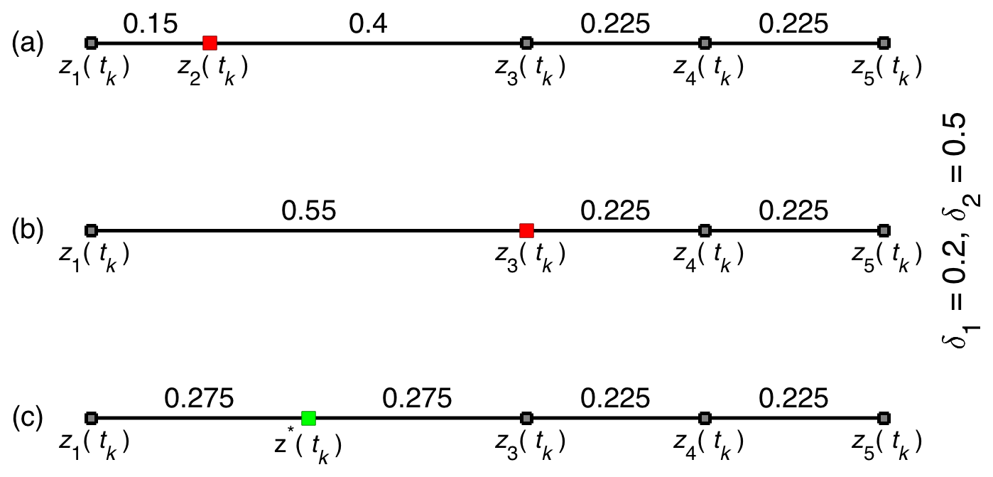
Figure 1An illustration of the remeshing process with δ1=0.2 and δ2=0.5: for invalid mesh (a), remove z2(tk), which violates δ1 (b), and insert z*(tk) to avoid violating δ2 (c).
The remeshing algorithm, with , is illustrated in Fig. 1 for the node z1(tk) at a particular time t=tk of the integration. The node z2(tk) has a distance of 0.15 from z1(tk), which is smaller than δ1; therefore, z2(tk) is removed (Fig. 1a). The next node, now z3(tk), has distance 0.55 from z1(tk), which exceeds δ2 (Fig. 1b); therefore, a new node, z*(tk), is introduced at the midpoint between z1(tk) and z3(tk) (Fig. 1c).
Figure 2 shows an example of this remeshing procedure applied to a velocity-based adaptive moving mesh using Burgers' equation (see Sect. 6 for details) as a physical model. We see how the nodes, oriented along the horizontal axis, follow a moving front. In particular, the mesh which initially has 40 equally distributed nodes ends up having only 27 unevenly distributed nodes as a result of the remeshing procedure.
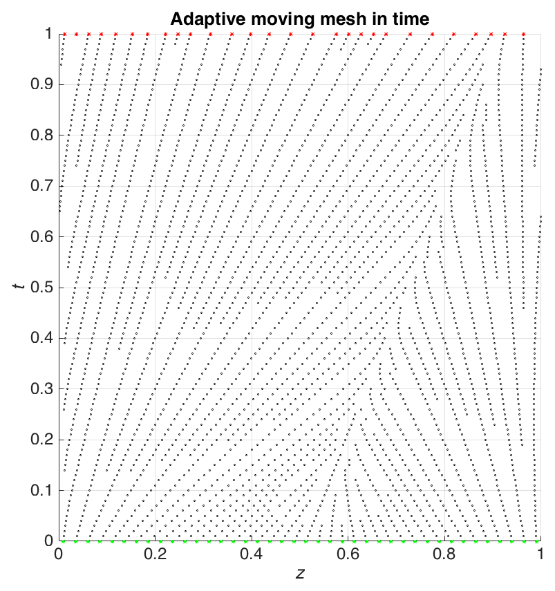
Figure 2An illustration of adaptive moving mesh over time solving Burgers' equation (see Sect. 6) until t=1 on a domain . In this example, the remeshing criteria are based on δ1=0.02 and δ2=0.05. There are 40 initial adaptive moving mesh nodes and 27 nodes at t=1; these are shown in green and red, respectively.
Since both the physical value(s) representing the system and the mesh on which the PDE is solved are evolved, we represent both in the state vector. The dimension of the state vector is then 2N, where N is the number of mesh nodes:
where the zi values are viewed as the mesh nodes and ui is the values of the physical variable u at zi.
The model will encompass all the algebraic relations of the computation, including the mesh advancement and remeshing. It need not be defined for every . Indeed, the mesh nodes will need to satisfy Eq. (3). We therefore introduce by the condition that when Eq. (3) holds.
The model operates between observation times. If we set t=tk as an observation time and as the next time at which observations will be assimilated, the model will be integrated with an adapting mesh, including Lagrangian evolution and possible multiple remeshings, from tk to tk+1. If xk=x(tk) then we set this model evolution as a map,
Note that if the original PDE (Eq. 1) is nonautonomous, i.e., f depends on t directly, then ℳ will depend on k and we would write ℳ=ℳk. For convenience, we assume that is a multiple of the computational time step. Moreover, we begin and end each integration between observation times with a remeshing if the given mesh is invalid. In this way, we guarantee that both zk and zk+1 can be taken to correspond to valid meshes. In principle, we can then apply ℳ to any element . Because of the tolerances δ1 and δ2, there are, however, constraints on N. Since they are both divisors of L, we can introduce N1 and N2 by
and we can restrict to . We can then view ℳ as acting on a larger space that puts all of its possible domains together. To this end, we set and, viewing each 𝕏N as distinct,
and cast ℳ as a mapping from 𝕏 to itself, i.e., , noting again that the N may change under this map, i.e., N may be different for xk and xk+1. In other words if , the next iteration is where, in general, .
We introduce a modification of the EnKF (Evensen, 2009) suitable for numerical models integrated on an adaptive moving mesh. The discussion herein pertains to the stochastic version of the EnKF (Burgers et al., 1998), but the approach can be straightforwardly extended to deterministic EnKFs (see, e.g., Sakov and Oke, 2008) without major modifications. A recent review on EnKF-like methods and their application to atmospheric circulation models can be found in Houtekamer and Zhang (2016).
The EnKF, originally introduced by Evensen (1994), is an ensemble-based formulation of the classical Kalman filter (KF) for linear dynamics (KF; Kalman, 1960). Like the KF, the EnKF is based on a Gaussian assumption for the error statistics in that they are fully described by the mean and covariance. The solution is obtained recursively by alternating a forecast step during which the state estimate and the associated error covariance are propagated in time and an analysis step in which the forecast state is combined with the observations. The analysis, which is viewed as the best possible estimate of the system's state, is obtained as the minimum variance estimator (see, e.g., Evensen, 2003). The EnKF computes the error statistics (i.e., mean and covariance) using an ensemble of model realizations (Evensen, 2003). The forward integration of the ensemble under the model dynamics replaces the explicit matrix multiplications involved in the forecast step of the KF. The EnKF, in conjunction with implementing localization and inflation (see, e.g., Carrassi et al., 2018, their Sect. 4.4 and references therein), has proved accurate in high-dimensional systems by using a number of ensemble members several orders of magnitude smaller than the system's dimension. The EnKF has led to dramatic computational savings over the standard KF and, importantly, does not require the model dynamics to be linear or linearized.
The challenge in implementing an EnKF on an adaptive moving mesh model with remeshing is that the dimension of the state vector will be potentially different for each ensemble member. This is addressed by Du et al. (2016) in which the idea of a fixed reference mesh, called observation mesh, is introduced which has higher resolution around the predefined observations. We will adopt this approach here but introduce a new variant in utilizing meshes of different resolutions. In particular, we will work with a high- and a low-resolution mesh. We see these as representing the extremes which should bracket the possible results of using meshes of various resolutions. They are, respectively, associated with the two tolerance parameters δ1 and δ2 and are therefore linked directly to the mesh of the models while giving us the flexibility of assimilating any type of observations without prior information, as is generally the case in realistic applications. In addition, in our approach, the analyzed states are mapped back onto the adaptive moving meshes to preserve the mesh, which resolves fine-scale structures generated by the dynamics of the models.
The location of the nodes and their total number are bound to change with time and across ensemble members: each member now provides a distinct discrete representation of the underlying continuous physical process based on a different number of differently located sample points. The individual ensemble members have to be intended now as samples from a different partition of the physical system's phase space, and they do not provide a statistically consistent sampling of the discrete-in-space uncertainty distribution. This is reflected in practice by the fact that the members cannot be stored column-wise any longer to form ensemble matrices, and thus the matrix computations involved in the EnKF analysis to evaluate the ensemble-based mean and covariance cannot be performed.
On the other hand, on the reference mesh, the members are all samples from the same discrete distribution and can thus be used to compute the ensemble-based mean and covariance. The entire EnKF analysis process is carried out on this fixed reference mesh, and the results are then mapped back to the individual ensemble meshes. This procedure amounts to the addition of two steps on top of those in the standard EnKF. First, we map each ensemble member from its adaptive moving mesh to an appropriate fixed uniform mesh and perform the analysis. Then, the updated ensemble members are mapped back to their adaptive moving meshes, providing the ensemble for the next forecast step.
The process is summarized schematically in Fig. 3. Steps S0 and S2, integration of the model ℳ to compute prior statistics, and the analysis step are common in an EnKF. At step S1, before the analysis, the forecast ensemble on adaptive moving meshes is mapped onto the fixed uniform mesh (Sect. 5.1), while step S3 amounts to the backward mapping from the fixed to the individual adaptive meshes. In the following sections, we give the details of processes in S1, S2 and S3, following their respective order in the whole DA cycle.

Figure 3Illustration of the analysis cycle in the proposed EnKF method for adaptive moving mesh models. In S1, adaptive moving meshes are mapped onto the fixed reference mesh. The ensemble is updated on the fixed reference mesh at step S2 (i.e., the analysis). Then, in S3 the updated ensemble members are mapped back to the corresponding adaptive moving meshes. The full process is illustrated in Fig. 4 for one ensemble member. See text in Sect. 5 for full details on the individual process steps, S0, S1, S2 and S3.
5.1 Fixed reference meshes
We divide the physical domain [0,L) into M cells of equal length, Δγ:
where . It follows that γ1=0 and for each i and that . Because of the periodicity, we identify 0 and L in the fixed mesh; in other words, . The points γi are the mesh nodes of the fixed reference mesh.
While we are, in principle, free to choose the fixed reference mesh arbitrarily, it makes sense to tailor it to the application under consideration. We choose to define the resolution of this fixed uniform mesh based on the maximum and minimum possible resolution of the individual adaptive moving meshes in the ensemble. The resolution range in the adaptive moving mesh reflects the computational constraints adapted to the specific physical problem: it therefore behooves us to bring these constraints into the definition of the fixed mesh for the analysis.
The high-resolution fixed reference mesh (HR) will be obtained by setting M=N1 and the low-resolution fixed reference mesh (LR) by setting M=N2. We will focus on these two particular fixed meshes, although the methodology described below could be adapted to working with any fixed reference mesh. Recalling that , and the criteria for a valid mesh given by Eq. (4), it can be seen that any valid mesh will have at most one node in each cell Li of an HR case and at least one node in each cell of an LR case. As will be seen below, the HR case will require some interpolation to fill in empty cells, whereas the LR case will average physical values at nodes that share a cell. It may seem that the higher-resolution mesh would always be preferable, but a key finding of this work is that this is not always true.
Note that the hypothesis , i.e., the tolerances δ1 and δ2 being divisors of the domain dimension L, does not need to be assumed. The computational and physical constraints of the model may suggest that δ1 and δ2 do not satisfy this condition; it would be a technical change in our method to accommodate such a situation.
5.2 Mapping onto a fixed reference mesh
The mapping will take a state vector , where is a valid mesh, onto a vector in with M=N1 (HR) or M=N2 (LR). The state vector to which the map is applied should be thought of as an ensemble member at the forecast step so that it has gone through remeshing after its final model evolution step. Thus N may be any integer between N1 and N2. This is step S1 in the scheme of Fig. 3.
We denote the mapping as , with M=N1 for j=1 (HR) or M=N2 for j=2 (LR) as above. Recalling that the γi are nodes of the fixed reference mesh, the image of specific x∈𝕏N values has the form
The physical value is viewed as the value of u at mesh node γi; the tilde is used hereafter to refer to quantities on the fixed reference mesh.
To set the u values, we introduce a shifted mesh as follows: set for , where δ=δ1 or δ2 and again M=N1 or N2, respectively. Furthermore, set . We view as an interval, since we identify 0 and L. The procedure is now separated into the high- and low-resolution cases.
Case 1 – HR. Taking x∈𝕏N as above, if there is a , then set . If there is no but zk<γi, then find k so that and set
If there is no such zk, then set
Case 2 – LR. For each i, find all values. Denote these as and set
The map 𝒫j is now well defined, in both the HR and LR cases, for each x∈𝕏N.
For the EnKF, we will also need the map that omits the mesh points in the fixed reference mesh,
and again M=N1 or N2 for HR or LR, respectively.
In the EnKF analysis, we will denote by and work with this reduced state vector, which consists only of the physical values and not the mesh points. A consequence is that we will not be updating the mesh locations but rather remapping the analysis back onto the original adaptive mesh for each ensemble member. We will discuss the possibility of updating the mesh locations in the conclusions.
5.3 Observation operator
The observations will be of physical values (u) at specific locations (zo). Assuming that there are d observations, then the observation operator will be a mapping on reduced state vectors given as i.e., , with M=N1 or N2. Each component of is the estimate the state vector gives of the observations at locations zo. For the explicit representation of the observation operator, let us consider one observation at once so that for all , we consider the jth observation and find i so that ; then the jth component of the observation operator reads
Since , this is the natural linear interpolation between values of u at γi and γi+1. The full observation operator is then
where each has the above form of an observation value at its respective observation locations .
Thus, we can eventually define the state vector on as
5.4 Analysis using the ensemble Kalman filter
After mapping all the ensemble members onto the dedicated fixed reference mesh (either the high- or the low-resolution one), the stochastic EnKF can be applied in the standard way. This is step S2 in our scheme. The mapped forecast ensemble members can be stored as columns on the forecast ensemble matrix,
with M=N1 or M=N2 for the HR and LR reference mesh, respectively, and Ne being the ensemble size. To simplify the notation the time index and the tilde from the matrices are omitted: all terms entering the analysis update operations are defined at the same analysis time onto the fixed, either HR or LR, mesh. The forecast ensemble mean is computed as
while the normalized forecast anomaly matrix Xf is formed by subtracting the forecast ensemble mean from each of the ensemble members as
Model outputs are confronted with the observations at the end of every analysis interval and are stored in the observation vector, y∈ℝd. The observations are related to the system state via the (generally nonlinear) observational model,
and are assumed to be affected by a Gaussian, zero-mean white-in-time noise ϵ with covariance , . In the experiments described in Sect. 7, we directly observe the model physical variables (onto the fixed reference mesh), , so that as explained in Sect. 5.3, the observation operator only involves a linear interpolation and is thus linear. Nevertheless, the approach described herein is suitable for working with nonlinear ℋ values subject to minor modifications.
In the stochastic EnKF (Burgers et al., 1998), the observations are treated as random variables so that each ensemble member assimilates a different perturbed observations vector,
with . We can now compute the normalized anomaly ensemble of the observations,
and define the ensemble-based observational error covariance matrix,
and the observed ensemble-anomaly matrix,
with and . The forecast ensemble member are then individually updated according to
where
is the ensemble-based Kalman gain matrix. It is worth recalling that in the limit, Ne→∞, Re→R and the Kalman gain, K converges to that of a classical, full-rank Kalman filter if both the dynamical and the observational models are linear and all of the errors are Gaussian.
When applied to large dimensional systems for which Ne≪M, as is typical in the geosciences, the success of the EnKF is related to the use of localization and inflation (see, e.g., Carrassi et al., 2018, their Sect. 4.4, for a review). In this work localization is not used, but the covariance multiplicative scalar inflation (Anderson and Anderson, 1999) is adopted so that the ensemble-based forecast anomaly matrix is inflated as
with α≥1, before Xf is used in the analysis update Eq. (27). Multivariate multiplicative inflation or more sophisticated adaptive inflation procedures exist and could have been implemented here, but this is not of great importance in this work, and the scalar coefficient α has been properly tuned. A recent review of adaptive inflation methods can be found in Raanes et al. (2019).
The updated analysis ensemble in Eq. (27) is then used to initialize the next forecast step. However, prior to this, we need to map back each individual analysis member on their respective adaptive, non-uniform mesh; the process is described in Sect. 5.5.
5.5 From a fixed reference mesh to an adaptive moving mesh
After the analysis, the update on the fixed reference mesh has to be mapped back onto the individual adaptive moving meshes of the ensemble members. In the forward mapping step S1 (see Fig. 3), the mapping indices associating the nodes in the adaptive moving mesh with nodes in the reference mesh are stored in an array. These are the indices resulting from the projections on the HR or the LR reference mesh as described in Sect. 5.2.
Each analysis ensemble member will thus retrieve its adaptive mesh from the stored array. In the reverse mapping step S3 (Fig. 3) the updated solution is projected to the adaptive moving meshes by locating each zj in an interval and assigning the mth component of to be the ith component of u in the vector xk that will initialize the model after the analysis time step.
In summary, each ensemble member after the analysis step will have the form
where if , then . The backward mapping procedure is the same for both HR and LR cases, although it will provide different results.
The process steps are illustrated in Fig. 4a and b, representing HR and LR cases, respectively, for one ensemble member, and using Burgers' equation as a model (Burgers, 1948); the model and experimental setup are described in detail in Sect. 6.
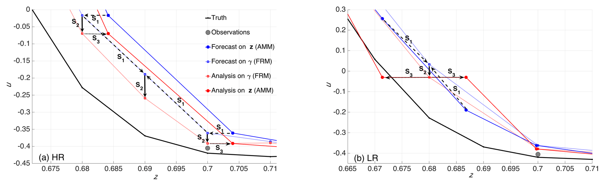
Figure 4Schematic illustration of the DA cycle on the high-resolution (a) and low-resolution (b) fixed reference mesh. On the legend, dark and light blue and red lines are forecast and analysis on adaptive moving mesh (AMM) and fixed reference mesh (FRM), respectively. Observations (gray circles) are sampled from the truth (black line). When following the arrows, S1 is the mapping the adaptive moving mesh onto the fixed reference mesh, S2 is update of the ensemble member and S3 is backward mapping onto the adaptive moving mesh (see Fig. 3).
Let consider first the HR case of Fig. 4a. In S1, the forecasted physical quantity uf on the adaptive moving mesh (dark blue with large circles) is mapped to the fixed reference mesh nodes (light blue with small circles) at and . The fixed mesh's node γm=0.69 is left emptied: a value is thus assigned by interpolation from the adjacent nodes . This provides the forecasted physical quantity, , on the full reference mesh and completes step S1. In the next step, S2, is updated using the stochastic EnKF as described in Sect. 5.4 to get the analysis field (light red line and small circles). Finally, in step S3, the is mapped back to the adaptive moving mesh so as to get ua (dark red line with large circles). Note that the physical quantity on the interpolated node γm in the fixed reference mesh is not mapped back (that node did not exist in the original adaptive mesh), yet it was required at step S2 to perform the analysis.
Similarly, Fig. 4b describes the LR case. In this situation, however, the forecasted physical quantity on the adaptive moving mesh nodes at 0.672 and 0.686 is averaged (step S1) in order to associate a value on the fixed reference mesh node γm=0.68 before the analysis. After the update (step S2), in step S3, the analysis at γm=0.68 is used to provide the analyses on both the original nodes (at 0.672 and 0.686) on the adaptive mesh that will have thus the same analyzed value. As a result of this, we observe that the analysis is better than the forecast (in the sense of being closer to the truth: compare dark blue and red circles, respectively, for forecast and analyses) at node z=0.672 but worse at node z=0.686. In this latter case in fact, the overestimate of the truth increases from about 0.15 to more than 0.3 for the forecast and analysis. On the other hand, at node z=0.672 the forecasted overestimate of about 0.2 is reduced to a slight underestimate of about 0.04.
We note a key aspect of our methodological choice: the ratio of the remeshing criteria exerts a control on the relation between the adaptive moving meshes and the fixed reference mesh. In fact, is the upper bound of the number of nodes that will be interpolated in the HR case and averaged in the LR case, since it represents the maximum ratio between the dimension of the fixed reference mesh and that a moving mesh can ever reach.
Our aim is to test the modified EnKF methodology described in Sect. 5 by performing controlled DA experiments with two numerical models and two types of synthetic observations: Eulerian and Lagrangian. In particular, we aim at assessing the impact and comparing the performance of the HR and LR options detailed in Sect. 5.
The first numerical model is the diffusive version of Burgers' equation (Burgers, 1948):
with periodic boundary conditions . In our experiments, we set the viscosity ν=0.08; the model Eq. (31) is hereafter referred to as BGM. Given that Burgers' equation can be solved analytically, it has been used in several DA studies (see, e.g., Cohn, 1993; Verlaan and Heemink, 2001; Pannekoucke et al., 2018).
As second model, we use an implementation of the Kuramoto–Sivashinsky equation (Papageorgiou and Smyrlis, 1991),
which is also given as periodic boundary conditions. Concentration waves, flame propagation and free surface flows are among the problems for which this equation is used. The higher-order viscosity, ν, is chosen as 0.027, which makes Eq. (32) display chaotic behavior (Papageorgiou and Smyrlis, 1991). Both numerical models are discretized using finite central differences and integrated with an Eulerian time-stepping scheme. We integrate them using very small time steps, 10−3 and 10−5 for BGM and KSM, respectively, since the equations are propagated forward explicitly. For the BGM, the remeshing criteria for mesh adaptation are δ1=0.01 and δ2=0.02, while they are δ1=0.02π and δ2=0.04π for the KSM. Given that the model domain has dimension L=1 and L=2π for BGM and KSM, respectively, this implies that the number of nodes in the HR and LR fixed reference mesh for the analysis is 100 and 50 for both BGM and KSM.
Two “nature runs” are obtained, one for each model, by integrating them on a high-resolution fixed uniform mesh. For both models, the meshes for the nature are intentionally chosen to be of at least the same resolution of the HR fixed uniform reference mesh of the analysis. The size of the nature run's mesh for the BGM is 100 (corresponding to a resolution of 0.01), while it is 120 for KSM (equivalent to a resolution of about 0.052).
We have limited the time length of the simulations in BGM to T=2, as the viscosity tends to dominate over longer times and dampen the wave motion. Figure 5a shows the nature run for BGM until T=2 with the initial condition
The figure shows clearly how the amplitude of the wave, picking around z=0.5 at initial time, is almost completely dampened out at the final time.
With the given choice of the viscosity, KSM is not as dissipative as BGM and simulations can be run for longer. KSM is initialized using
as the initial condition. Then, it is spun up until T=20, and the solution at T=20 is used as the initial condition for the DA experiments. Figure 5b shows the KSM nature run until t=5 after re-initialization of the model following the spin-up (i.e., the actual simulation time being ); the chaotic behavior of the KSM solution can be qualitatively identified by the random oscillations.
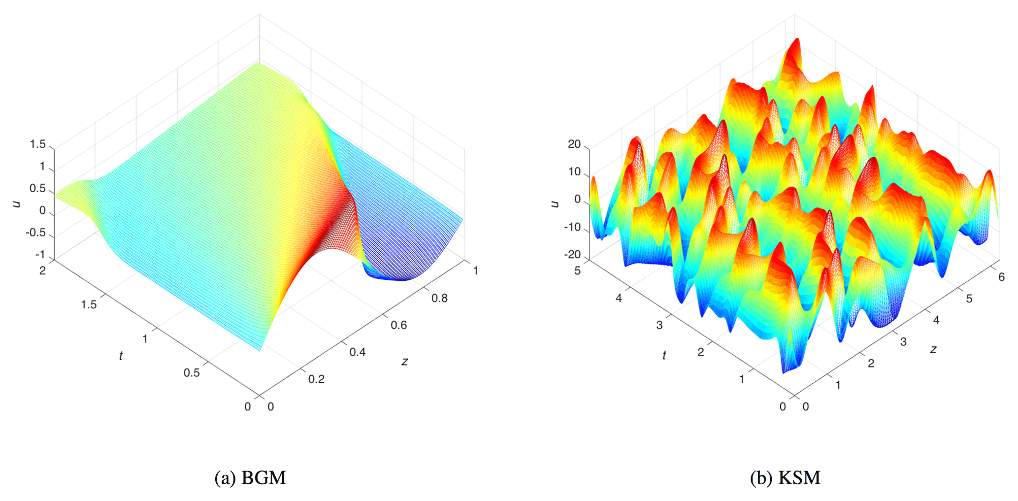
Figure 5Numerical solutions of Burgers' and Kuramoto–Sivashinsky equations. The solutions are computed on an uniform fixed mesh and represent the nature run from which synthetic Eulerian and Lagrangian observations are sampled.
Synthetic Eulerian and Lagrangian observations are sampled from the nature run. Eulerian observations are always collected at the same, fixed-in-time locations of the domain. We assume that Eulerian observers are evenly distributed along the one-dimensional domain (i.e., observations are at equally spaced locations) and that their total number is constant, so the number of observations at time step tk is for all k>0. The locations of the Lagrangian observations, on the other hand, change in time: the data are sampled by following the trajectories, solutions of the model. Being advected by the flow, Lagrangian observations may eventually concentrate within a small area of the model domain; they can thus be more spatially localized compared to Eulerian observations. In our experiments with Lagrangian observations, if two observations come within the threshold distance, 10−3, the one closer to the upper boundary of the spatial domain is omitted from the assimilation at that time and all future observation times so as not to oversample a specific location. As a result, the total number of Lagrangian observations will tend to decrease in time. An illustration of the different spatial coverage provided by the Eulerian and Lagrangian observations is given in Fig. 6 for the BGM with on the mesh of the nature run.
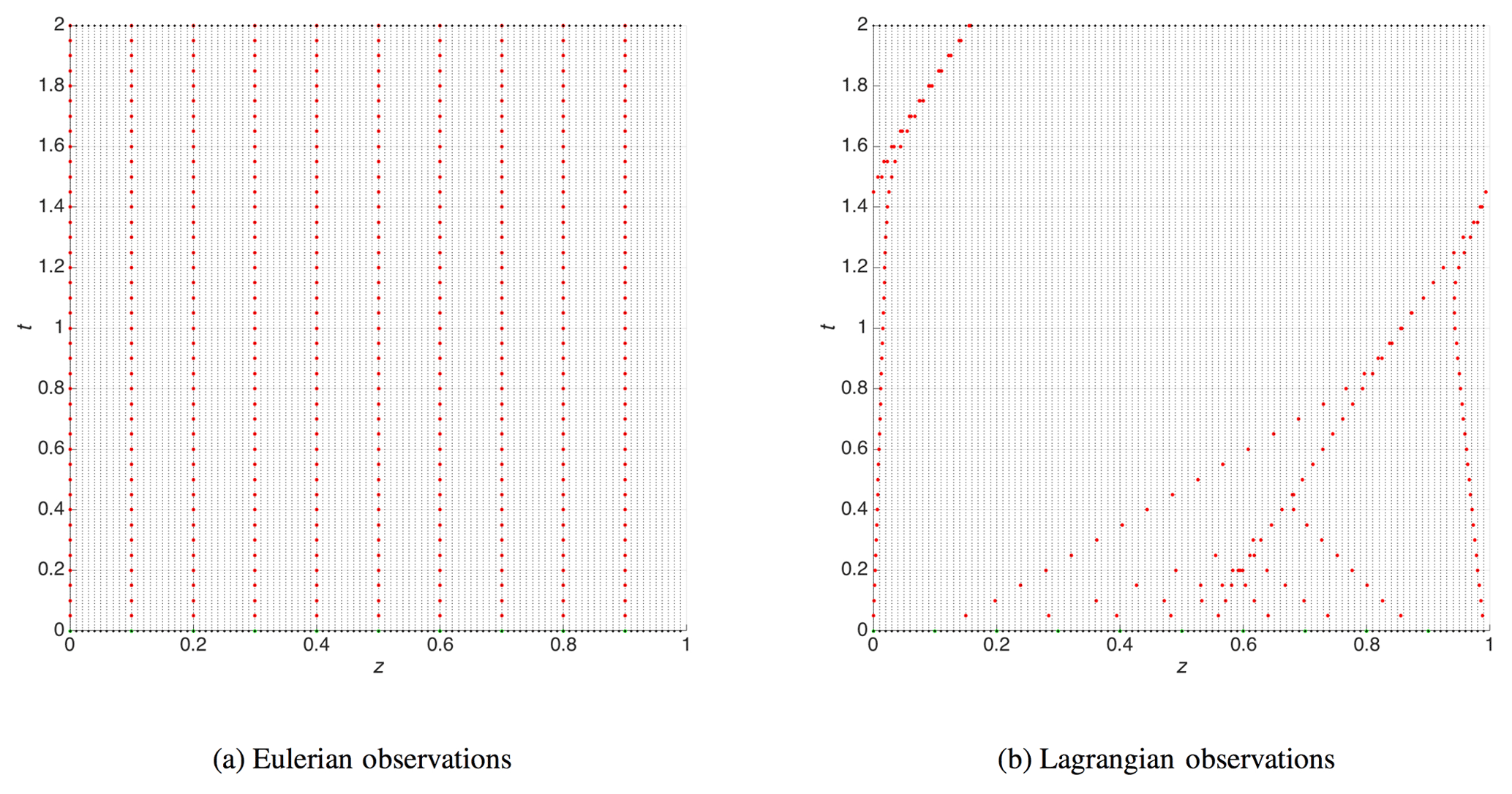
Figure 6Observations sampled from the BGM nature run (see Fig. 5a) in Eulerian (a) and Lagrangian (b) manner, mimicking geostationary satellite and buoy measurements, respectively.
In the experiments that follow, we chose to deploy as many Lagrangian observers at t0 as Eulerian ones and to place them at the same locations, i.e., d0=d. The number of Eulerian observations and the initial number of Lagrangian observations is set to and for BGM and KSM, respectively. Gaussian, white-in-time and spatially uncorrelated noise is added to these observations; the observational error covariance matrix is diagonal so that , with σo being the observational error standard deviation and I being the identity matrix. These synthetic observations are assimilated with the modified EnKF presented in Sect. 5.4, and the specifications of its implementation, namely the number of initial ensemble members, initial mesh size and inflation, are provided in the Sect. 7. The analysis interval is set to Δt=0.05 time units in all the DA experiments and for both models and observation types. A summary of the experimental setup is given in Table 1.
Table 1Experimental setup parameters: ν is the viscosity, δ1 and δ2 the remeshing criteria, N1 and N2 are the number of nodes in the HR and LR fixed reference mesh, T is the duration of the experiments, Δt is the analysis interval, and dEUL and are the number of Eulerian observations and the initial number of Lagrangian observations.
The experiments are compared by looking at the root-mean-square error (RMSE) of the ensemble mean (with respect to the nature run) and the ensemble spread. Since the analysis is performed on either the HR or the LR fixed mesh, the computation of the RMSE and spread is done on the mesh resulting from their intersection. Given that we have chosen the remeshing criteria in both models such that δ1 is half of δ2, the intersection mesh is the LR mesh itself. Finally, in all of the experiments, the time mean of the RMSE and spread are computed after T=1 time units, unless stated otherwise.
We present the results in three subsections. In Sect. 7.1 and 7.2, we investigate the modified EnKF with fixed reference mesh (either HR or LR) for the BGM and KSM, respectively, using Eulerian observations. In these sections we also present the tuning of the EnKF with respect to the ensemble size (Ne), inflation factor (α) and initial adaptive moving mesh size (N0). The combination of those parameters giving the best performance with BGM is then kept and used in Sect. 7.3, where the comparison between Eulerian and Lagrangian observations cases is described.
7.1 Modified EnKF for adaptive moving mesh models – Burgers' equation
In this section, the experiments using BGM are presented. In order to calculate the base error due to the choice of the specific fixed reference mesh, HR or LR, and the resulting mapping procedures, we first perform an ensemble run without assimilation. This DA-free ensemble run is subject to all of the steps described in Fig. 3, except for step S2, in which the analysis update is performed. Given that DA is not carried out, the difference between the HR and LR experiments (if any) can only be due to the mapping procedures. Recall that this procedure differs in that it involves interpolation or averaging in the HR or LR cases, respectively. For consistency, the mapping to or from the fixed reference mesh is performed every , i.e., the time between the assimilation of observations.
Figure 7 displays the RMSE and the ensemble spread for the HR and LR in these DA-free ensemble runs. We see that the RMSE is slightly larger in the LR than in the HR case, indicating that averaging introduces larger errors than interpolation in this specific model scenario. This can be interpreted in terms of the sharpness of Burgers' solution (see Fig. 5a) that might not be accurately described using the LR mesh. Furthermore, this is also consistent with what is observed in Fig. 4b, in which the LR analysis was deteriorating the forecast in some instances. After an initial faster error growth in the LR case, at about t=0.4, the difference between LR and HR almost stabilizes, with the two error curves having the same profile. The ensemble spread is initially slightly larger in the HR case, but it then attains similar values for both HR and LR after t=0.6, suggesting that the spread does not depend critically on the type of mapping and resolutions of the fixed reference mesh. While this appears to be a reasonable basis for building the EnKF, Fig. 7 also highlights the undesirable small spread of values compared with the RMSE. We will come back to this point in the DA experiments to follow.
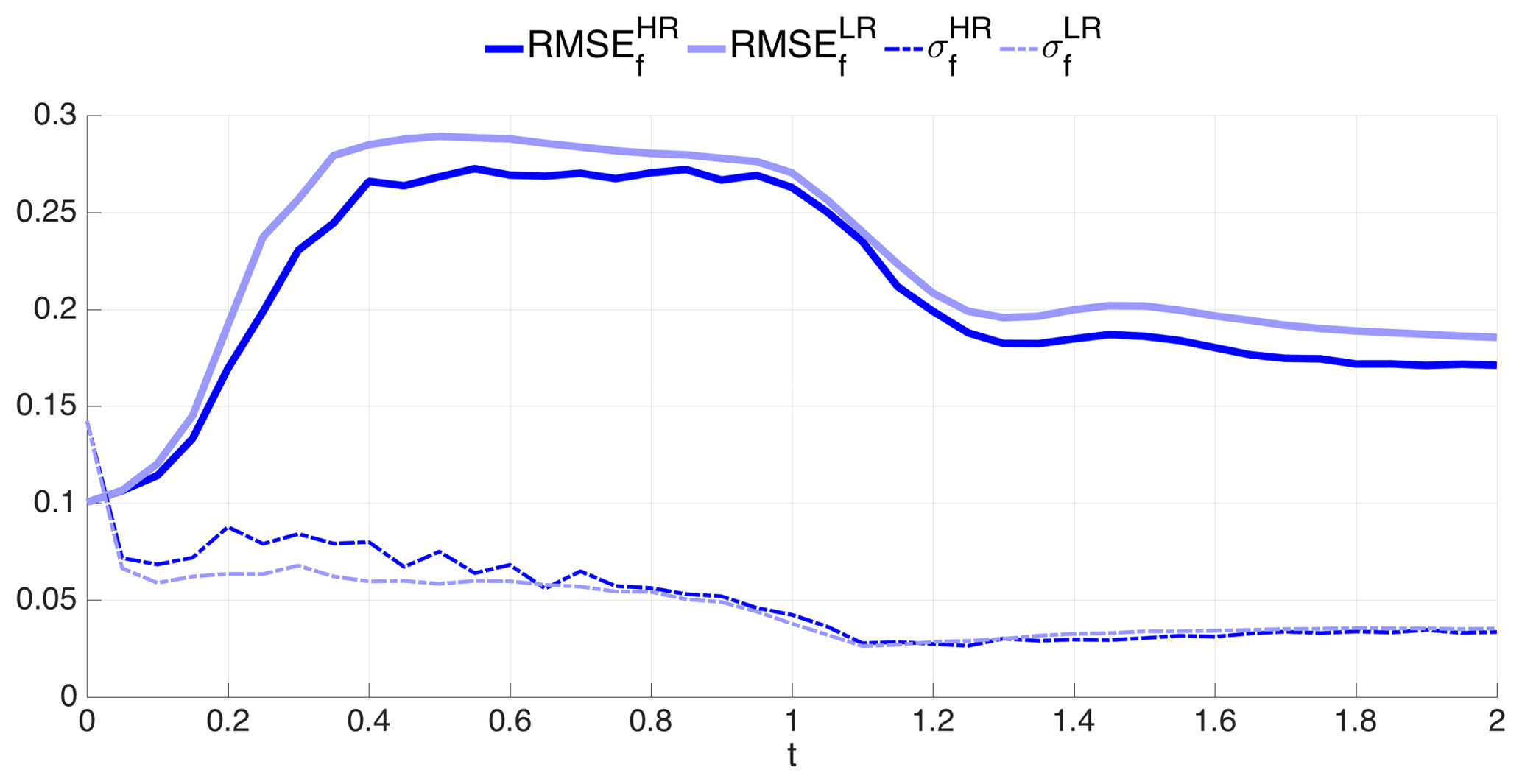
Figure 7Time evolution of the forecast RMSE (solid line) and spread (σ; dashed line) of DA-free ensemble run using BGM. Dark and light blue lines represent the HR and LR, respectively.
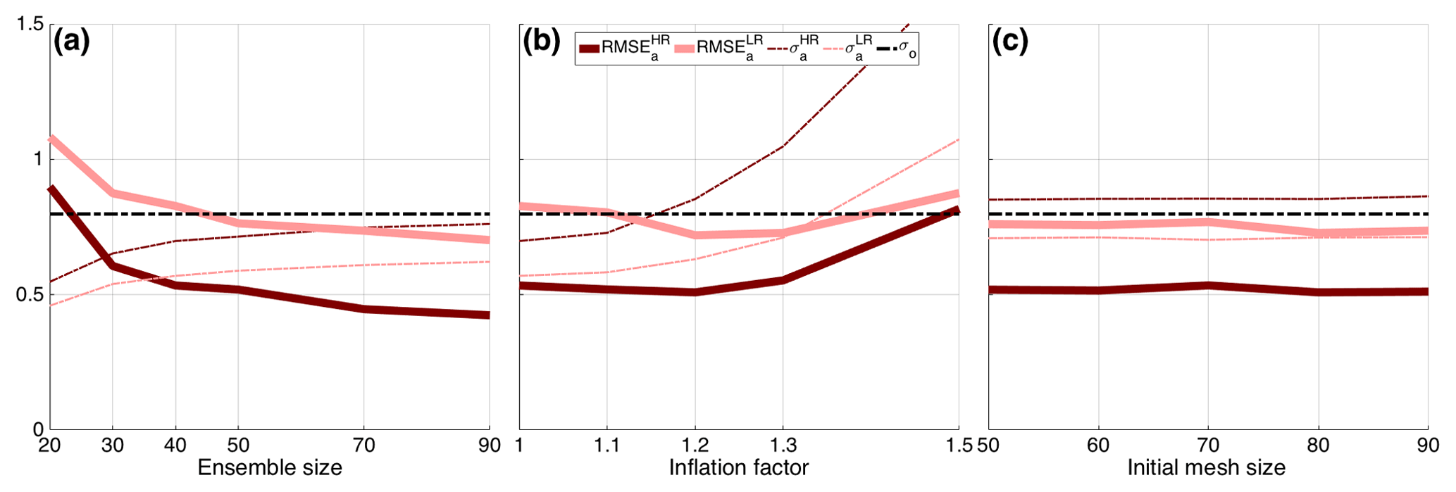
In the DA experiments, we study the sensitivity of the EnKF to the ensemble size, inflation factor and initial size of the adaptive moving meshes. Recall that the ensemble members are all given the same uniform mesh at the initial time; however these meshes will then inevitably evolve into a different, generally non-uniform mesh for each member. We remark that the three parameters under consideration are all interdependent, and a proper tuning would involve varying them simultaneously, which would make the number of experiments grow too much. To reduce the computational burden, we opted instead to vary only one at a time while keeping the other two fixed.
The results of this tuning are displayed in Fig. 8, which shows the RMSE of the EnKF analysis (the ensemble mean), and the spread, as a function of the ensemble size, inflation factor and initial mesh size, respectively, in Fig. 8a, b and c. The RMSE and spread are averaged in space and time after the initial spin-up period T=1. For reference, we also plotted the observational error standard deviation (horizontal black dashed line).
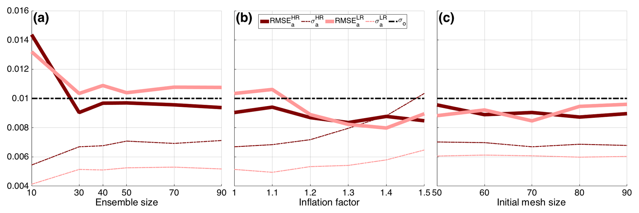
Figure 8Time mean of the RMSE of the analysis ensemble mean (solid line) and ensemble spread (σ; dashed line) of BGM for different ensemble size, Ne (a), inflation factor, α (b), and initial mesh size, N0 (c). Dark and light red lines show the HR and LR, respectively.
In the case of the sensitivity to the ensemble size (Fig. 8a), Ne is varied between 10 and 90, while the initial mesh size is kept to 70 for both HR and LR cases, and inflation is not used (i.e., α=0). The RMSE in the HR case is generally lower than in the LR case; it is, respectively, slightly below and above the observational error standard deviation. In both cases, however, the RMSE approximately converges to quasi-stationary values as soon as Ne≥30. This phenomenon, which we also observe for KSM in the next section, is reminiscent of the behavior in a chaotic system, where the EnKF error converges when Ne is larger or equal to the dimension of the unstable–neutral subspace of the dynamics (Bocquet and Carrassi, 2017).
We therefore set Ne=30 and study the sensitivity to the inflation factor in Fig. 8b (the initial mesh size is still kept to 70). Inflation is expected to mitigate the difference (the underestimation) between the RMSE and the spread shown in Fig. 8a. By looking at Fig. 8b this seems actually to be the case, and in the LR case the RMSE and spread decrease and increase by increasing the inflation factor α. In the HR case, the RMSE is already lower than the observational standard deviation and the inflation has only a small effect: the increase in spread is not accompanied by a similar decrease in error. Based on this, we hereafter set the inflation to α=1 and α=1.45 for HR and LR, respectively.
Finally, in Fig. 8c, we consider the initial mesh size; recall that the ensemble size is set to Ne=30. Also recall that the size of the individual member's adaptive moving mesh size, N, is controlled by the remeshing tolerances δ1=0.01 and δ2=0.02 and can vary throughout the integration between 50 and 100. In the set of experiments depicted in Fig. 8c, we initialize the ensemble on an adaptive moving mesh of size N0, ranging from 50 to 90. Interestingly, the EnKF does not exhibit great sensitivity to N0, and the differences between HR and LR appear to be very small and not systematic. The fact that LR kept the RMSE at the level of the HR is the result of successful tuning. We saw in fact that the mapping error in the LR case is larger (see Fig. 7). Nevertheless this initial disadvantage of the LR has been largely compensated by the inflation. In the experiments that follow, we have chosen to fix N0=70 for both HR and LR.
The results of the tuning experiments of Fig. 8 and selected values of the parameters are reported in Table 2 and are used in the experiments of Fig. 9, which shows the forecast and analysis RMSE and spread for both HR and LR as a function of time. Notably the HR and LR perform quite similarly for t>1.2, when the solution of the model is possibly of small amplitude due to the viscous damping. Nevertheless, for t≤1.2, LR is often as good as (t<0.4) or better () than HR, making LR a viable, computationally more economic solution. The time-averaged RMSE and spread of these experiments are included in Table 2.
Table 2Ensemble size (Ne), inflation factor (α) and initial mesh size (N0) chosen from the sensitivity experiments in Fig. 8 to perform the experiment in Fig. 9. Resulting time mean of the RMSE and spread (σ) in for the HR and LR using BGM between t=0 and t=2 are also listed.
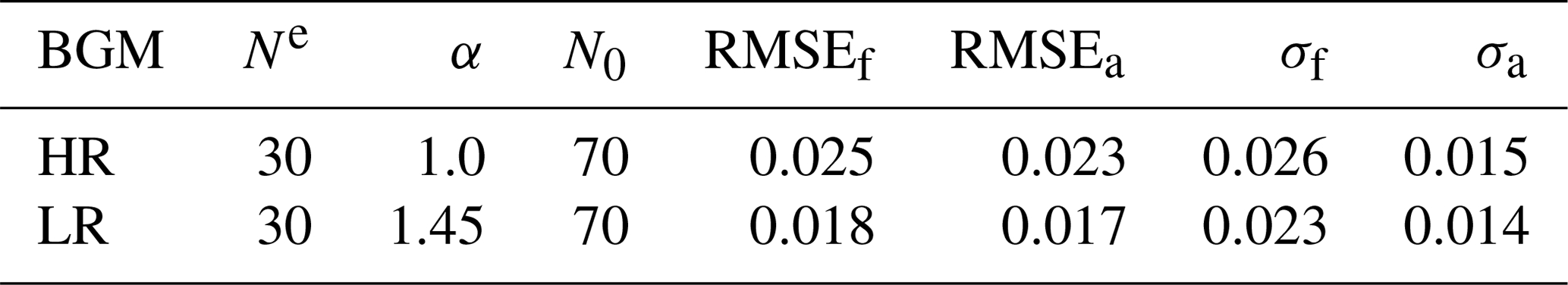
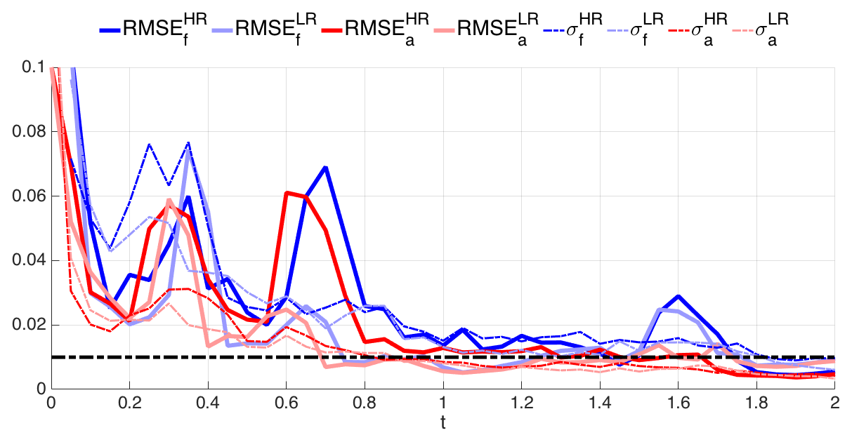
Figure 9Time evolution of the RMSE (solid line) and spread (σ, dashed line) for BGM until t=2. Dark and light lines represent the HR and LR, respectively. Blue and red lines show forecast and analysis, respectively.
7.2 Modified EnKF for adaptive moving mesh models – Kuramoto–Sivashinsky equation
This section shows the same type of results as in the previous section, this time being applied to the KSM. We begin by evaluating the errors related to the mapping on the HR and LR case by running a DA-free ensemble; results are shown in Fig. 10.

As opposed to what is observed in Fig. 7, we see now that the different mapping procedures in the HR and LR cases induce similar errors and impact the spread in a similar way. This difference is certainly due to the different dynamical behavior in BGM and KSM, with the solution of the latter displaying oscillations over all of the model domain. These can be in some instances well represented (i.e., less affected) by the averaging procedure in the LR case and in others by the interpolation in the HR case. Another remarkable difference with respect to BGM is that now the ratio spread and RMSE is larger, meaning that the spread underestimates the RMSE relatively less than for BGM.
Figure 11 shows the same set of experiments as in Fig. 8, this time using KSM. The time mean of the RMSE and spread are again considered after t=1, but experiments are run until t=5, since KSM is not as dissipative as BGM with chosen values for the viscosity. Furthermore, all values are normalized using an estimate of the model internal variability based on the spin-up integration from t=0 to (see Sect. 6).
In Fig. 11a, the analysis RMSE and spread are shown against the ensemble size, Ne. No inflation is applied, and initial mesh size is chosen to be 80 in both the HR and LR cases. The analysis RMSE goes below the observation error standard deviation as soon as Ne=30 in the HR case, but an ensemble as big as Ne=50 is required in the LR case. Based on these results, we have chosen to use Ne=40 for both cases as a trade-off between computational cost and accuracy, given that the RMSE in the LR case is very close to observational accuracy. Notably, the spread is quite large in both cases and is even larger than the RMSE in the HR configuration. With Ne=40, the impact of inflation is considered in Fig. 11b. We see here how the spread is consistently increased by increasing the inflation factor α and the corresponding RMSEs decrease until α=1.3 and increase afterwards, possibly as a consequence of too much spread. The selected values for the inflation factor are α=1.2 and 1.3 for the HR and LR cases, respectively. Fig. 11c studies the sensitivity to the initial mesh size, N0. Similarly to what is observed for the BGM in Fig. 8c, the performance of the EnKF does not show a marked sensitivity to N0: it is arguable that the mesh size of the individual members quickly adjusts to the values with little memory of the initial dimension. In the experiments that follow, the initial mesh size is set to N0=80 in both HR and LR configurations. Overall Fig. 11 indicates that, as opposed to BGM, with KSM, the EnKF on the HR fixed reference mesh is always superior to the LR fixed mesh. The selected optimal values of Ne, α and N0 are reported in Table 3.
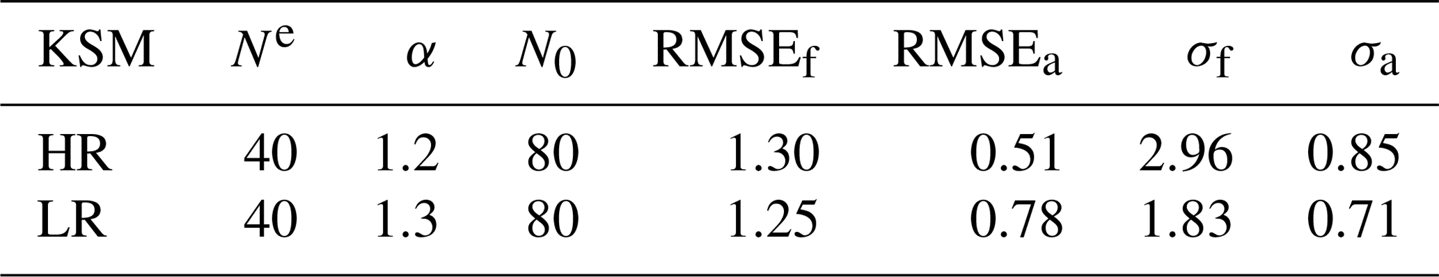
Figure 12 shows the time evolution of the forecast and analysis RMSE and spread for HR and LR until t=5 using these selected values. First, we observe that the analysis RMSE is always lower than the corresponding RMSE of the forecast in both the HR and the LR cases. Remarkably the spread of the forecast is also larger than the RMSE of the forecast, in both configurations, pointing to healthy performance of the EnKF. As for the comparison between HR and LR we see that now the former is systematically better than the latter, suggesting that in the KSM, the benefits of performing the analysis on HR are larger compared to BGM. Nevertheless, the LR case also performs well, and it could be preferred when computational constraints are taken into consideration. The time-averaged RMSEs and spreads are reported in Table 3.
7.3 Impact of observation type: Eulerian versus Lagrangian
Up to this point, we have only utilized Eulerian observations. Using the optimal setup presented in the previous sections, we now assess the impact of different observation types, i.e., Eulerian or Lagrangian (see Figs. 6a and 6b). We consider here only the BGM with the LR configuration for the fixed reference mesh, and the values for the experimental parameters are those in Table 2 (first three columns of the second row). Results (not shown) with the KSM using Lagrangian observations indicate that the EnKF was not able to track the true signal, possibly as a consequence of the Lagrangian observers ending trapped within only few of the many fronts in the KSM solution (see Fig. 5b): the number of observations and their distribution then becomes insufficient.
Figure 13 shows the forecast and analysis RMSE as a function of time for both Eulerian and Lagrangian data. As for previous figures, the observation error standard deviation is superimposed as reference, but the number of Lagrangian observers is now included (right y axis). Recall that Lagrangian data are bound to decrease with time (see Sect. 6 and Fig. 6b) and that their initial number and locations are the same as for the Eulerian observations, i.e., , and they are equally spaced.
At first sight, one can infer from Fig. 13 that overall Lagrangian data are approximately as effective as their Eulerian counterparts even though they are fewer in number. This is reminiscent of a known advantage of Lagrangian observations that has been documented in a number of studies (see, e.g., Kuznetsov et al., 2003; Nodet, 2006; Apte and Jones, 2013; Slivinski et al., 2015, and references therein); however the actual positions at which the observations are made are assimilated in these pieces of work. A closer inspection of Fig. 13 reveals also other aspects. For instance, it is remarkable that between , the assimilation of Lagrangian observations is superior to using fixed, evenly distributed Eulerian ones. On the other hand, when t≥1.3, the assimilation of Eulerian data is always better than Lagrangian, a behavior possibly due to the fact that and that, despite their dynamically guided locations, there are not as many as required to properly keep the error low. It is finally worth pointing out the episode of the very high analysis RMSE (higher than the corresponding forecast RMSE) occurring at t=1.5: the assimilation was in that case clearly detrimental. Nevertheless the EnKF was quickly able to recover, and the RMSE is reduced to much smaller values, close to the observation error.


Figure 13Time evolution of the RMSE until t=2 using BGM. Light blue and red lines are the forecast and analysis RMSE with the Eulerian observations, respectively. Dark blue and gray lines are the same as the Lagrangian observations. Gray dashed line shows the number of Lagrangian observations in time.
We propose a novel methodology to perform ensemble data assimilation with computational models that use non-conservative adaptive moving mesh. Meshes of this sort are said to be adaptive because their node locations adjust to some prescribed rule that is intended to improve model accuracy. We have focused here on models with a Lagrangian solver in which the nodes move following the model's velocity field. They are said to be non-conservative because the total number of nodes in the mesh can itself change when the mesh is subject to remeshing. We have considered the case in which remeshing avoids having nodes too close or too far apart than given tolerance distances; in practice the tolerances define the set of valid meshes. When an invalid mesh appears through integration, it is then remeshed and a valid one is created.
The major challenge for ensemble data assimilation stands in that the dimension of the state space changes in time and differs across ensemble members, impeding the normal ensemble-based operations (i.e., matrix computations) at the analysis update. To overcome this issue, we have added in our methodology one forward and one backward mapping step before and after the analysis, respectively. This mapping takes all the ensemble members onto a fixed, uniform reference mesh. On this mesh, all ensemble members have the same dimension and are defined onto the same spatial mesh; thus the assimilation of data can be performed using standard EnKF approaches. We have used the stochastic EnKF, but the approach can be easily adapted to the use of a square-root EnKF. After the analysis, the backward mapping returns the updated values to the individual, generally different and non-uniform meshes of the respective ensemble members.
We consider two cases: a high-resolution and a low-resolution fixed uniform reference mesh. The essential property is that their resolution is determined by the remeshing tolerances δ1 and δ2 such that the high- and low-resolution fixed reference meshes are the uniform meshes that bound, from above and below, respectively, the resolution of all relevant adaptive meshes. While one can in principle use a fixed reference mesh of arbitrary resolution, our choice connects the resolution of the reference mesh to the given physical and computational constraints, reflected by the tolerance values in the model design. This in practice means that our reference mesh cell will contain at most, or at least, one node of the ensemble member mesh in either the high- or low-resolution cases, respectively. Hence, using this characterization, we can avoid excessive smoothing or interpolation at the mapping stages. Depending on whether the tolerances are divisors of the model domain dimension, the reference meshes can also be themselves valid meshes; nevertheless this condition is not required for the applicability of our approach.
We tested our modified EnKF using two 1-D models, the Burgers and Kuramoto–Sivashinsky equations. A set of sensitivity tests is carried through some key model and DA setup parameters: the ensemble size, inflation factor and initial mesh size. We considered two types of observations: Eulerian and Lagrangian. It is shown that, in general, a high-resolution fixed reference mesh improves the estimate more than a low-resolution fixed reference mesh. Whereas this might indeed be expected, our results also show that a low-resolution reference mesh affords a very high level of accuracy if the EnKF is properly tuned for the context. The use of a low-resolution fixed mesh has the obvious advantage of a lower computational burden, given that the size of the matrix operations is to be implemented at the analysis step scales with the size of the fixed reference mesh.
We then examined the impact of assimilating Lagrangian observations compared with Eulerian ones and have seen, in the context of Burgers equation, that the former improves the solution as much as the latter. The effectiveness of Lagrangian observers, despite being fewer in number than for the case of fixed, Eulerian observations, comes from their concentrating, where their information is most useful, i.e., within the sharp single (shock-like) front of the Burgers solution.
In this work, we have focused on the design of the strategy and, for the sake of clarity, have focused only on updating the physical quantities, while the locations of the ensemble mesh nodes were left unchanged. A natural extension of this study is to subject both the model physical variables and the mesh locations to the assimilation of data. Both would then be updated at the analysis time, and this is currently under investigation.
This paper is part of a longer-term research effort aimed at developing suitable EnKF strategies for a next-generation 2-D sea-ice model of the Arctic Ocean, neXtSIM, which solves the model equations on a triangular mesh using finite element methods and a Lagrangian solver. The velocity-based mesh movement and remeshing procedure that we have built into our 1-D model scenarios were formulated with the aim of mimicking those specific aspects of neXtSIM. In terms of our different types of observations, the impact of Eulerian and Lagrangian observational data was studied in light of observations gathered by satellites and drifting buoys, respectively, which are two common observing tools for Arctic sea ice.
Such a 2-D extension is, however, a non-trivial task for a number of fundamental reasons. First of all, given the triangular unstructured mesh in neXtSIM, we cannot straightforwardly define an ordering of the nodes on the adaptive moving mesh, as is done in the 1-D case considered here. As a consequence, the determination of a fixed reference mesh might not be linked to the remeshing criteria in the same straightforward way. However, it is still possible to define a high- or low-resolution fixed reference mesh with respect to the mesh of neXtSIM, since the remeshing in neXtSIM is mainly used to keep the initial resolution throughout the integration. Secondly, the models considered in this study are proxies of continuous fluid flows, whereas the rheology implemented in neXtSIM treats the sea ice as a solid brittle material which results in discontinuities when leads and ponds form due to fracturing and ice melting; the Gaussian assumptions implicit in the EnKF formulation then need to be reconsidered. Nevertheless, the methodology presented in this study, and the experiments herein, confronts some of the key technical issues of the 2-D case. The current results in 1-D are encouraging regarding the applicability of the proposed modification of the EnKF to adaptive moving mesh models in two dimensions, and the extension to two dimensions is the subject of the authors' current research.
No data sets were used in this article.
The methodology has been developed by all of the authors. AA and CG coded and ran the experiments. The paper has been edited by all authors.
The authors declare that they have no conflict of interest.
The authors are thankful to Laurent Bertino for his comments and suggestions. We are thankful also to the editor and three anonymous referees for their constructive reviews.
Ali Aydoğdu, Alberto Carrassi and Pierre Rampal have been funded by the project REDDA (no. 250711) of the Norwegian Research Council. Alberto Carrassi and Pierre Rampal have also benefitted from funding from the Office of Naval Research project DASIM II (award N00014-18-1-2493). Colin T. Guider and Chris K. R. T. Jones have been funded by the Office of Naval Research award N00014-18-1-2204.
This paper was edited by Wansuo Duan and reviewed by three anonymous referees.
Alharbi, A. and Naire, S.: An adaptive moving mesh method for thin film flow equations with surface tension, J. Comput. Appl. Math., 319, 365–384, https://doi.org/10.1016/j.cam.2017.01.019, 2017. a
Anderson, J. L. and Anderson, S. L.: A Monte Carlo implementation of the nonlinear filtering problem to produce ensemble assimilations and forecasts, Mon. Weather Rev., 127, 2741–2758, 1999. a
Apte, A. and Jones, C. K. R. T.: The impact of nonlinearity in Lagrangian data assimilation, Nonlin. Processes Geophys., 20, 329–341, https://doi.org/10.5194/npg-20-329-2013, 2013. a
Asch, M., Bocquet, M., and Nodet, M.: Data Assimilation: Methods, Algorithms, and Applications, Fundamentals of Algorithms, SIAM, Philadelphia, ISBN 978-1-611974-53-9, 2016. a
Babus̆ka, I. and Aziz, A.: On the Angle Condition in the Finite Element Method, SIAM J. Numer. Anal., 13, 214–226, https://doi.org/10.1137/0713021, 1976. a
Baines, M. J., Hubbard, M. E., and Jimack, P. K.: Velocity-Based Moving Mesh Methods for Nonlinear Partial Differential Equations, Commun. Comput. Phys., 10, 509–576, https://doi.org/10.4208/cicp.201010.040511a, 2011. a, b
Berger, M. J. and Oliger, J.: Adaptive mesh refinement for hyperbolic partial differential equations, J. Comput. Phys., 53, 484–512, https://doi.org/10.1016/0021-9991(84)90073-1, 1984. a
Bishop, C. H., Etherton, B. J., and Majumdar, S. J.: Adaptive sampling with the ensemble transform Kalman filter. Part I: Theoretical aspects, Mon. Weather Rev., 129, 420–436, 2001. a
Bocquet, M. and Carrassi, A.: Four-dimensional ensemble variational data assimilation and the unstable subspace, Tellus A, 69, 1304504, https://doi.org/10.1080/16000870.2017.1304504, 2017. a
Bonan, B., Nichols, N. K., Baines, M. J., and Partridge, D.: Data assimilation for moving mesh methods with an application to ice sheet modelling, Nonlin. Processes Geophys., 24, 515–534, https://doi.org/10.5194/npg-24-515-2017, 2017. a, b, c
Bouillon, S. and Rampal, P.: Presentation of the dynamical core of neXtSIM, a new sea ice model, Ocean Model., 91, 23–37, https://doi.org/10.1016/j.ocemod.2015.04.005, 2015. a
Bouillon, S., Rampal, P., and Olason, E.: Sea Ice Modelling and Forecasting, in: New Frontiers in Operational Oceanography, edited by: Chassignet, E. P., Pascual, A., Tintoré, J., and Verron, J., 15, 423–444, GODAE OceanView, https://doi.org/10.17125/gov2018, 2018. a
Budhiraja, A., Friedlander, E., Guider, C., Jones, C., and Maclean, J.: Assimilating data into models, in: Handbook of Environmental and Ecological Statistics, edited by: Gelfand, A. E., Fuentes, M., Hoeting, J. A., and Smith, R. L., ISBN 9781498752022, CRC Press, 2018. a
Burgers, G., Jan van Leeuwen, P., and Evensen, G.: Analysis scheme in the ensemble Kalman filter, Mon. Weather Rev., 126, 1719–1724, https://doi.org/10.1175/1520-0493(1998)126<1719:ASITEK>2.0.CO;2, 1998. a, b
Burgers, J.: A Mathematical Model Illustrating the Theory of Turbulence, vol. 1 of Advances in Applied Mechanics, 171–199, Elsevier, https://doi.org/10.1016/S0065-2156(08)70100-5, 1948. a, b
Carrassi, A., Bocquet, M., Bertino, L., and Evensen, G.: Data assimilation in the geosciences: An overview of methods, issues, and perspectives, Wiley Interdisciplinary Reviews: Climate Change, 9, e535, https://doi.org/10.1002/wcc.535, 2018. a, b, c, d
Cohn, S. E.: Dynamics of short-term univariate forecast error covariances, Mon. Weather Rev., 121, 3123–3149, 1993. a
Compère, G., Remacle, J. F., and Marchandise, E.: Transient Mesh Adaptivity with Large Rigid-Body Displacements, in: Proceedings of the 17th International Meshing Roundtable, edited by: Garimella, R., 213–230, Springer, Berlin, 2008. a
Compère, G., Remacle, J.-F., Jansson, J., and Hoffman, J.: A mesh adaptation framework for dealing with large deforming meshes, Int. J. Numer. Meth. Engng., 82, 843–867, https://doi.org/10.1002/nme.2788, 2009. a
Dansereau, V., Weiss, J., Saramito, P., and Lattes, P.: A Maxwell elasto-brittle rheology for sea ice modelling, The Cryosphere, 10, 1339–1359, https://doi.org/10.5194/tc-10-1339-2016, 2016. a
Davies, D. R., Wilson, C. R., and Kramer, S. C.: Fluidity: A fully unstructured anisotropic adaptive mesh computational modeling framework for geodynamics, Geochem. Geophy. Geosy., 12, 6, https://doi.org/10.1029/2011GC003551, 2011. a, b
Du, J., Zhu, J., Fang, F., Pain, C., and Navon, I.: Ensemble data assimilation applied to an adaptive mesh ocean model, Int. J. Numer. Meth. Fl., 82, 997–1009, https://doi.org/10.1002/fld.4247, 2016. a, b, c, d
Evensen, G.: Sequential data assimilation with a nonlinear quasi-geostrophic model using Monte Carlo methods to forecast error statistics, J. Geophys. Res.-Oceans, 99, 10143–10162, https://doi.org/10.1029/94JC00572, 1994. a
Evensen, G.: The ensemble Kalman filter: Theoretical formulation and practical implementation, Ocean Dynam., 53, 343–367, https://doi.org/10.1007/s10236-003-0036-9, 2003. a, b
Evensen, G.: Data Assimilation: The Ensemble Kalman Filter, Springer-Verlag/Berlin/Heildelberg, second edn., ISBN 978-3-642-03711-5, 2009. a, b, c
Fang, F., Piggott, M., Pain, C., Gorman, G., and Goddard, A.: An adaptive mesh adjoint data assimilation method, Ocean Model., 15, 39–55, https://doi.org/10.1016/j.ocemod.2006.02.002, 2006. a
Farrell, P., Piggott, M., Pain, C., Gorman, G., and Wilson, C.: Conservative interpolation between unstructured meshes via supermesh construction, Comput. Meth. Appl. Mech. Eng., 198, 2632–2642, https://doi.org/10.1016/j.cma.2009.03.004, 2009. a
Houtekamer, P. L. and Zhang, F.: Review of the Ensemble Kalman Filter for Atmospheric Data Assimilation, Mon. Weather Rev., 144, 4489–4532, https://doi.org/10.1175/MWR-D-15-0440.1, 2016. a, b
Huang, W. and Russell, R. D.: Adaptive moving mesh methods, vol. 174, Springer Science & Business Media, ISBN 978-1-4419-7916-2, 2010. a, b, c, d, e
Huang, W., Zheng, L., and Zhan, X.: Adaptive moving mesh methods for simulating one-dimensional groundwater problems with sharp moving fronts, International J. Numer. Meth. Eng., 54, 1579–1603, https://doi.org/10.1002/nme.482, 2002. a
Jain, P. K., Mandli, K., Hoteit, I., Knio, O., and Dawson, C.: Dynamically adaptive data-driven simulation of extreme hydrological flows, Ocean Model., 122, 85–103, https://doi.org/10.1016/j.ocemod.2017.12.004, 2018. a
Kalman, R. E.: A new approach to linear filtering and prediction problems, J. Fluid. Eng., 82, 35–45, 1960. a
Kuznetsov, L., Ide, K., and Jones, C.: A method for assimilation of Lagrangian data, Mon. Weather Rev., 131, 2247–2260, 2003. a
Maddison, J., Marshall, D., Pain, C., and Piggott, M.: Accurate representation of geostrophic and hydrostatic balance in unstructured mesh finite element ocean modelling, Ocean Model., 39, 248–261, https://doi.org/10.1016/j.ocemod.2011.04.009, 2011. a
Marsan, D., Stern, H. L., Lindsay, R., and Weiss, J.: Scale dependence and localization of the deformation of Arctic sea ice, Phys. Rev. Lett., 93, 178501, https://doi.org/10.1103/PhysRevLett.93.178501, 2004. a
Nodet, M.: Variational assimilation of Lagrangian data in oceanography, Inverse problems, 22, 245, https://doi.org/10.1088/0266-5611/22/1/014, 2006. a
Pain, C., Piggott, M., Goddard, A., Fang, F., Gorman, G., Marshall, D., Eaton, M., Power, P., and de Oliveira, C.: Three-dimensional unstructured mesh ocean modelling, Ocean Model., 10, 5–33, https://doi.org/10.1016/j.ocemod.2004.07.005, 2005. a
Pannekoucke, O., Bocquet, M., and Ménard, R.: Parametric covariance dynamics for the nonlinear diffusive Burgers equation, Nonlin. Processes Geophys., 25, 481–495, https://doi.org/10.5194/npg-25-481-2018, 2018. a
Papageorgiou, D. T. and Smyrlis, Y. S.: The route to chaos for the Kuramoto-Sivashinsky equation, Theor. Computat. Fluid Dynam., 3, 15–42, 1991. a, b
Partridge, D.: Numerical modelling of glaciers: moving meshes and data assimilation, PhD thesis, University of Reading, 2013. a
Raanes, P. N., Bocquet, M., and Carrassi, A.: Adaptive covariance inflation in the ensemble Kalman filter by Gaussian scale mixtures, Q. J. Roy. Meteor. Soc., 145, 53–75, https://doi.org/10.1002/qj.3386, 2019. a
Rabatel, M., Rampal, P., Carrassi, A., Bertino, L., and Jones, C. K. R. T.: Impact of rheology on probabilistic forecasts of sea ice trajectories: application for search and rescue operations in the Arctic, The Cryosphere, 12, 935–953, https://doi.org/10.5194/tc-12-935-2018, 2018. a
Rampal, P., Weiss, J., Marsan, D., Lindsay, R., and Stern, H.: Scaling properties of sea ice deformation from buoy dispersion analysis, J. Geophys. Res.-Oceans, 113, C03002, https://doi.org/10.1029/2007JC004143, 2008. a
Rampal, P., Bouillon, S., Ólason, E., and Morlighem, M.: neXtSIM: a new Lagrangian sea ice model, The Cryosphere, 10, 1055–1073, https://doi.org/10.5194/tc-10-1055-2016, 2016. a, b, c
Rampal, P., Dansereau, V., Olason, E., Bouillon, S., Williams, T., and Samaké, A.: On the multi-fractal scaling properties of sea ice deformation, The Cryosphere Discuss., https://doi.org/10.5194/tc-2018-290, in review, 2019. a
Sakov, P. and Oke, P. R.: A deterministic formulation of the ensemble Kalman filter: an alternative to ensemble square root filters, Tellus A, 60, 361–371, 2008. a
Saksono, P. H., Dettmer, W. G., and Perić, D.: An adaptive remeshing strategy for flows with moving boundaries and fluid-structure interaction, Int. J. Numer. Meth. Eng., 71, 1009–1050, https://doi.org/10.1002/nme.1971, 2007. a
Slivinski, L., Spiller, E., Apte, A., and Sandstede, B.: A hybrid particle–ensemble Kalman filter for Lagrangian data assimilation, Mon. Weather Rev., 143, 195–211, 2015. a
Talagrand, O.: Assimilation of Observations, an Introduction (Special Issue – Data Assimilation in Meteology and Oceanography: Theory and Practice), J. Meteorol. Soc. Jpn., 75, 191–209, 1997. a
Verlaan, M. and Heemink, A. W.: Nonlinearity in Data Assimilation Applications: A Practical Method for Analysis, Mon. Weather Rev., 129, 1578–1589, https://doi.org/10.1175/1520-0493(2001)129<1578:NIDAAA>2.0.CO;2, 2001. a
Weller, H., Ringler, T., Piggott, M., and Wood, N.: Challenges Facing Adaptive Mesh Modeling of the Atmosphere and Ocean, B. Am. Meteorol. Soc., 91, 105–108, https://doi.org/10.1175/2009BAMS2907.1, 2010. a
- Abstract
- Introduction
- The physical model and its integration
- A one-dimensional, non-conservative velocity-based adaptive moving mesh
- The model state and its evolution
- The ensemble Kalman filter for an adaptive moving mesh model
- Experimental setup
- Results
- Conclusions
- Data availability
- Author contributions
- Competing interests
- Acknowledgements
- Financial support
- Review statement
- References