Particle clustering and subclustering as a proxy for  mixing in geophysical flows

Chakraborty, Rishiraj; Coutino, Aaron; Stastna, Marek

doi:https://doi.org/10.5194/npg-26-307-2019

Articles | Volume 26, issue 3

https://doi.org/10.5194/npg-26-307-2019

Articles | Volume 26, issue 3

Research article

16 Sep 2019

Research article |

| 16 Sep 2019

Particle clustering and subclustering as a proxy for mixing in geophysical flows

Rishiraj Chakraborty, Aaron Coutino, and Marek Stastna

Abstract

The Eulerian point of view is the traditional theoretical and numerical tool to describe fluid mechanics. Some modern computational fluid dynamics codes allow for the efficient simulation of particles, in turn facilitating a Lagrangian description of the flow. The existence and persistence of Lagrangian coherent structures in fluid flow has been a topic of considerable study. Here we focus on the ability of Lagrangian methods to characterize mixing in geophysical flows. We study the instability of a strongly non-linear double-jet flow, initially in geostrophic balance, which forms quasi-coherent vortices when subjected to ageostrophic perturbations. Particle clustering techniques are applied to study the behavior of the particles in the vicinity of coherent vortices. Changes in inter-particle distance play a key role in establishing the patterns in particle trajectories. This paper exploits graph theory in finding particle clusters and regions of dense interactions (also known as subclusters). The methods discussed and results presented in this paper can be used to identify mixing in a flow and extract information about particle behavior in coherent structures from a Lagrangian point of view.

Download & links

Article (PDF, 2822 KB)

How to cite

How to cite.

Dates

Received: 24 Feb 2019 – Discussion started: 14 Mar 2019 – Revised: 03 Jul 2019 – Accepted: 26 Jul 2019 – Published: 16 Sep 2019

1 Introduction

There are two different geometric approaches to fluid mechanics, the Eulerian and the Lagrangian approach. In the Eulerian approach, field values are obtained on a spatial grid, for example from numerical simulation output. In the Lagrangian approach measurement data are obtained following the fluid, as in the case of temperature measurements by a weather balloon. Many naturally occurring flows are complex, three-dimensional and, at least to some extent, turbulent. Such flows are characterized by a richness of vorticity and the rapid mixing of passive tracers as discussed in (Davidson, 2015, chap. 3). At the same time, satellite imagery suggests that large-scale flows exhibit prominent coherent patterns, and this is theoretically supported by the so-called inverse cascade of two-dimensional turbulence in which energy moves to larger scales while enstrophy moves to smaller scales (Davidson, 2015, chap. 10).

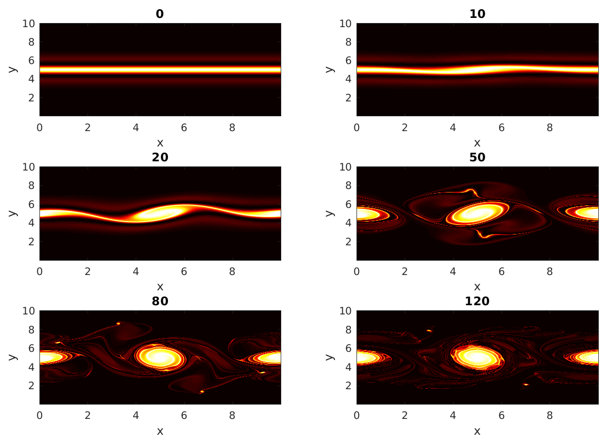
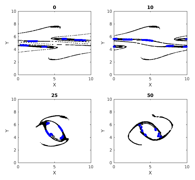
https://www.nonlin-processes-geophys.net/26/307/2019/npg-26-307-2019-f01

Figure 1The enstrophy field showing the evolution of the unstable double jet with time. The bright areas indicate regions of high enstrophy which are found between the two jets at early times.

Download

Even three-dimensional turbulent flows are known to contain quasi-deterministic coherent structures (Hussain, 1983). Coherent structures can be thought of as turbulent fluid masses having temporal correlation in vorticity over some spatial extent (e.g., a shear layer in a flow). Figure 1 shows the evolution of the enstrophy field of a two-dimensional double jet initially in geostrophic balance, subjected to ageostrophic perturbations. The evolution depicts the formation of vortices due to instability of the geostrophic flow. Coherent structures like vortices and filaments undergo frequent stretching and folding. The identification of coherent structures in turbulent flows gave the revolutionary notion in fluid mechanics that turbulent flows are not completely random but can contain orderly organized structures, and these coherent structures in specific regions can influence mixing, transport and other physically relevant features (Kline et al., 1967).

The study of coherent flow structures has received significant interest in the recent past. The existing methods for detecting coherent behavior mathematically are either geometric or probabilistic; Allshouse and Peacock (2015) discuss and compare the different methods. Geometric methods aim to find distinct boundaries between the coherent structures, whereas probabilistic methods use the concept of sets with minimal dispersion moving in a flow to identify coherent structures. Padberg-Gehle and Schneide (2017) in their introduction, however, note that existing methods for finding coherent structures require the full knowledge of the flow field and the underlying dynamical system. This, in turn, requires high-resolution trajectory data. This can be numerically expensive as well as challenging to find in applications. Hadjighasem et al. (2017), in their review of various Lagrangian techniques for finding coherent structures, say that the Lagrangian diagnostic scalar field methods are incapable of providing a strict definition of coherent flow structures and are also not effective in establishing a precise mathematical connection between the geometric features and the flow structures. Such diagnostic methods include the finite-time Lyapunov exponent (FTLE), finite-size Lyapunov exponent (FSLE), mesochronic analysis, trajectory length, trajectory complexity and shape coherence. Hadjighasem et al. (2017) also describe the various methods of applying mathematical coherence principles to locate coherent structures. However, these principles only apply for finite-time intervals from the beginning of the flow evolution; it is not guaranteed that the coherence principles comply with observed coherent patterns at later times. Examples of mathematical coherence principles include transfer operator methods like the probabilistic transfer operator (Froyland, 2013) and the dynamic Laplace operator (Froyland, 2015). These methods identify maximally coherent or minimally dispersive (not dispersive in the sense of wave theory) regions over a finite-time interval. Such regions are expected to minimally mix with the surrounding phase space and are named “almost-invariant sets” for autonomous systems and “coherent sets” for non-autonomous systems. A different mathematical approach is the hierarchical coherent pairs method (Froyland et al., 2010), which initially splits a given domain into a pair of coherent sets using the transfer operator method and then subsequently refines the coherent sets iteratively. This is accomplished using the probabilistic transfer operator. The iteration is carried out until a reference measure of the probability, μ, falls below a user-defined cutoff. A third category of mathematical approaches for finding coherent structures based on Lagrangian data is clustering. Hadjighasem et al. (2017) reviews the fuzzy C-means clustering of trajectories by Froyland and Padberg-Gehle (2015), which uses the traditional fuzzy C-means clustering to identify finite-time-coherent structures and mixing in a flow. This method uses trajectories of Lagrangian particles over discrete time intervals and applies the fuzzy C-means algorithm to locate coherent sets as clusters of trajectories according to the dynamic distances between trajectories. Another similar method for locating coherent structures is the spectral clustering of trajectories, as proposed by Hadjighasem et al. (2016) and implemented by Padberg-Gehle and Schneide (2017). Mancho et al. (2004) discusses algorithms to compute hyperbolic trajectories from data sets on oceanographic flows and how to locate their stable and unstable manifolds. Mendoza and Mancho (2010) also discuss how phase portraits obtained using Lagrangian descriptors can provide a representation of the interconnected features of the underlying dynamical system. Rose et al. (2015) uses a coupled implementation of a mix of Eulerian and Lagrangian models for simulating the full life cycles of fish species anchovy and sardine in the California Current systems. The Lagrangian model used is an individual fish-based model which tracks each fish of every species. Padberg-Gehle and Schneide (2017) used a generalized graph Laplacian eigenvalue problem to extract coherent sets from several fabricated examples (e.g., Bickley jet) as well as measured data. The authors also highlighted regions of strong mixing in flow, using local network measures like node degree and the local clustering coefficient. These local network measures provide information for each Lagrangian particle.

Inspired by these, we wish to extract regions of dense mixing in flow using a graph theoretic network approach and compare the results with those obtained from spectral clustering. We also wish to use an evolving simulation for which coherent regions evolve dynamically through stretching and folding and are not known a priori. The trajectory encounter volume idea of Rypina and Pratt (2017) is similar to our methodology, but the volume in which particles are pre-identified is chosen based on features that are assumed to be already present in the flow (i.e., eddies). Moreover, the authors state that the method breaks down for sparse grids, since it is dependent on being able to define an effective density of particles. Detailed comparison with our method is thus left to future work.

From an Eulerian point of view, mixing can be characterized by studying the advection–diffusion equation for a passive tracer θ (Salmon, 1998),

\begin{matrix} (1) & \frac{\partial θ}{\partial t} + v \cdot \nabla θ = κ \nabla^{2} θ, \end{matrix}

where v is the fluid velocity and κ is the diffusion coefficient. Mixing and stirring depends on the gradient of θ, and hence the extent of mixing and stirring in a given domain for a given flow can be measured by the spatial variability index

\begin{matrix} (2) & C = \frac{1}{2} \int \int \nabla θ \cdot \nabla θ d x . \end{matrix}

Taking the time derivative of C, and following the simplification procedure in Salmon (1998), we obtain

\begin{matrix} (3) & \frac{d C}{d t} = \int \int [(v \cdot \nabla θ) \nabla^{2} θ - κ (\nabla^{2} θ)^{2}] d x . \end{matrix}

Fundamentally, mixing is a result of molecular diffusion, and hence the diffusive (second) term in Eq. (3) represents the effect of mixing, while the first term containing the gradient of θ represents the effect of stirring. This implies that an initial high value of ∇θ will promote mixing and hence diffusion, which in turn will to lead to a decrease in ∇θ. This can also be verified from a dynamical system's point of view. Prants (2014), in his review paper, describes mixing as follows. Let us consider the basin A with a circulation where there is a domain B with a dye occupying, at t=0, the volume V(B₀). Let us consider a domain C in A. The volume of the dye in the domain C at time t is V(B_t∩C), and its concentration in C is given by the ratio $V (B_{t} \cap C) / V (C)$ . Full mixing is defined in the sense that in the course of time, for any domain C∈A, the concentration of the dye is the same as in every other region in A. However, calculating the true three-dimensional Eulerian flow field, and the distribution of θ, for an actual geophysical flow (e.g., a hurricane) is an impossible task. This is due to the immense range of scales that typifies naturally occurring fluid motions. If one considers a hurricane, active scales range from hundreds of kilometers to sub-millimeter scales. Many models in geophysical fluid dynamics thus focus on representing the coherent scales of motion. In such cases the fundamentally three-dimensional motions that would carry out efficient mixing are filtered out during the theoretical derivation of the governing equations. A Lagrangian approach to mixing, based on particle proximity, may thus be more profitable. This is because it allows for an idealized representation of the three-dimensional turbulence that is ignored by the governing equations.

Klimenko (2009) provides an example of this approach to describe mixing. His idea is stochastic, where each particle has a deterministic component of motion governed by the known flow field and a random walk component. The particles are assigned scalar properties which can change due to mixing. The random walk component depends on the joint probability distribution of the particle as functions of position and the scalar properties. In his equation (36) the author defines the intensity of mixing between two particles as proportional to the distance between the particles in physical space. Inspired by Klimenko (2009), we use a numerically inexpensive version of this idea by loosely saying that there is some non-zero probability of mixing with exchange of properties taking place between two particles that approach below a given threshold, and a qualitative measure of mixing is given by interaction among particles. Interaction, once occurred, is counted as a unit of mixing, and our hypothesis says that if we have three particles, say, A, B and C, and if particle A interacts with particle B and if particle B interacts with particle C, then, indirectly, particle A has interacted with particle C to some extent. We then extend this idea to the assumption that a region comprising of a higher number of interacting particles corresponds to one with higher probabilities of mixing. The technical details are discussed in Sect. 2.3.

The remaining parts of the paper are structured in the following manner. Section 2 discusses the methods used in our work including the governing equations and description of the numerical code used to solve them. This is followed by the methods for clustering particles (Sect. 2.2), identifying regions of mixing (Sect. 2.3) and the methods for spectral clustering (Sect. 2.4). Section 3 presents a detailed discussion of the results obtained by implementing each of the methods above and also draws relevant comparisons as needed. The final section, Sect. 4, concludes the work and highlights the major findings.

2 Methods

2.1 Governing equations and numerical methods

We consider the shallow water equations on the f-plane (Kundu et al., 2008). All simulations are carried out with a code developed in house using CUDA, called CUDA Shallow Water and Particles (cuSWAP), which provides numerical solutions to the shallow water equations. CUDA is a parallel computing platform based on C, developed by NVIDIA to harness the computational power of GPUs (graphics processing units; Garland et al., 2008). We choose to solve these equations using spectral methods to take advantage of the cuFFT library (NVIDIA Corporation, 2010). This code solves the governing equations in a doubly periodic domain with variable topography. The input–output is handled using NETCDF. The time-stepping scheme is the low-memory Huen method (Ascher and Petzold, 1998). This code also has a Lagrangian attribute which performs particle tracking using cubic interpolation and symplectic Euler time stepping (Al-Kahby et al, 2000). Additionally this code dynamically calculates and outputs neighbors of a particle based on inter-particle distance. These data represent particle interactions and are used to construct adjacency matrices relevant to our work, as described in Sect. 2.2.

The shallow water equations, written out in the form amenable to numerical solution with an FFT-based (FFT – fast Fourier transform) method, express the conservation of mass,

\frac{\partial η}{\partial t} + (H + η) (\frac{\partial u}{\partial x} + \frac{\partial v}{\partial y}) + u (\frac{\partial H}{\partial x} + \frac{\partial η}{\partial x}) + v (\frac{\partial H}{\partial y} + \frac{\partial η}{\partial y}) = 0,

and the conservation of linear momentum,

\begin{array}{l} \frac{\partial u}{\partial t} + u \frac{\partial u}{\partial x} + v \frac{\partial u}{\partial y} - f v = - g \frac{\partial η}{\partial x}, \\ \frac{\partial v}{\partial t} + u \frac{\partial v}{\partial x} + v \frac{\partial v}{\partial y} + f u = - g \frac{\partial η}{\partial y}, \end{array}

where $η (x, y, t)$ is the perturbation height field, H(x,y) is the bottom topography (taken as constant throughout the present work), $(u (x, y, t), v (x, y, t))$ is the velocity field, f is the rotation rate taken as constant (i.e., the f-plane) and g is the acceleration due to gravity. The pressure field is hydrostatic.

The initial conditions consist of a geostrophically balanced jet and an ageostrophic perturbation with a radially symmetric form. The exact functional form of the perturbation was not found to be important for triggering the instability of the jet. The functional form of the initial conditions is given by

\begin{array}{l} u (x, y, 0) = 2 g a_{0} \frac{\tanh (y)}{\cosh^{2} (y)}, \\ v (x, y, 0) = 0, \\ η (x, y, 0) = a_{0} (\frac{1}{\cosh^{2} (y)} + \frac{1}{\cosh^{8} (\sqrt{x^{2} + y^{2}} / 2)}), \end{array}

where a₀=0.1H₀. The two relevant dimensionless numbers are the Froude number and Rossby number,

\begin{array}{l} Fr = \frac{U}{\sqrt{g H}} \approx 0.17, \\ Ro = \frac{U}{f L} \approx 0.3775 . \end{array}

Results will be reported in dimensionless form. The simulation is thus carried out in a square domain with side dimension 10. The resolution used is 2048×2048, and the number of particles tracked is 400×400, initially distributed uniformly in a grid pattern. The resolution is fine enough to represent both the primary, vortex-generating instability and the filaments formed from the interaction between vortices. We carried out a number of resolution checks, and indeed the 2048×2048 grid over-resolves the relevant phenomena. A decrease of a factor of 4 leaves the results essentially unchanged. While mixing is a small-scale phenomenon, it is not believed the results reported below are affected by the numerical discretization. Moreover, on a grid of fixed side, the spectral method employed is very close to the optimal numerical method available. Indeed a far more serious question down the line is how to represent the transition from large-scale, nearly two-dimensional flow to three-dimensional flow; this is a change that would require a fundamental shift in the software used.

2.2 Clustering particles

Clustering the particles in a flow means that we group the particles based on some form of particle behavior we wish to identify. In this paper we target the phenomenon of mixing in a flow by measuring instances of particle–particle proximity below a threshold. The inter-particle interactions we employ fall under the category of binary classification, i.e., two particles have either interacted or they have not. We set a threshold inter-particle distance ϵ such that at some given time, if the distance between any two particles becomes less than ϵ, those two particles will be said to have interacted with each other at that time. For mixing, it is natural to demand that the value of ϵ is less than grid spacing (though note that Padberg-Gehle and Schneide, 2017, in fact demand ϵ to be greater than the grid spacing for spectral clustering). Thus, for every time step, we search for particles which are within a radial distance of ϵ from every particle. A natural mathematical way to represent this information is to build a matrix. These matrices are known as adjacency matrices, which are symmetric square matrices with dimensions (number of particles squared). Each row in an adjacency matrix corresponds to a particle, and the columns correspond to all the particles that this particle may interact with. If particle “i” is said to have interacted with particle “j”, then the adjacency matrix, an initially zero matrix, will be 1 in cells (i,j) and (j,i). Figure 2 demonstrates a tutorial example of how to construct an adjacency matrix from particle interactions. There are two ways in which we create an adjacency matrix in our work:

Cumulative adjacency matrix. One interaction between two particles in the entire time span will yield a permanent 1 in the corresponding cells of the particles in the matrix.
Instantaneous adjacency matrix. One interaction between two particles at a particular time will yield a temporary 1 in the corresponding cells of the particles in the matrix. This type of matrix is refreshed every output time, and new 1s and 0s are registered for the new output time.

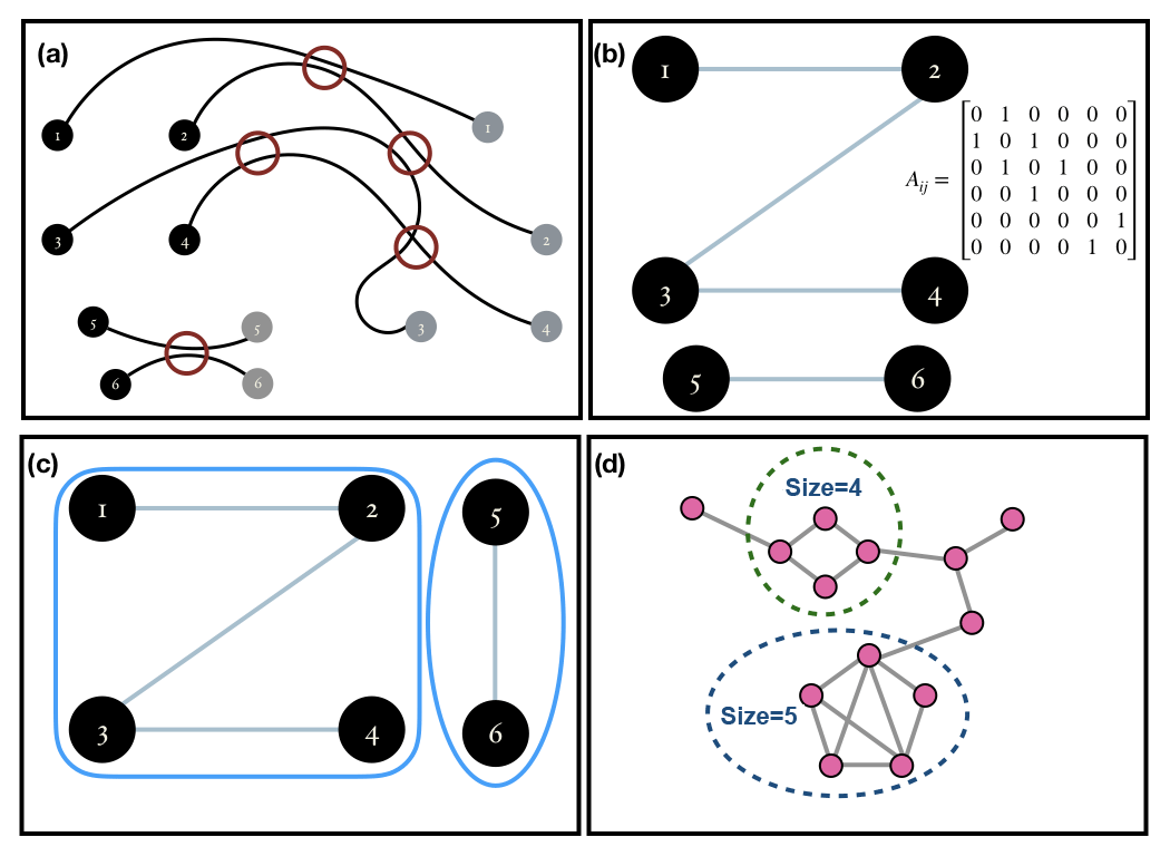
https://www.nonlin-processes-geophys.net/26/307/2019/npg-26-307-2019-f02

Figure 2(a) Idealized Lagrangian paths of six particles, showing where they have interacted along the course of their paths. (b) Adjacency matrix and graph corresponding to the particle interactions shown in (a). (c) Graph split into its connected components. (d) A connected graph symbolizing a scaled-down version of a cumulative cluster; the black dotted circles denote the dense sub-graphs for an arbitrary min_size=3 and γ=0.4.

Download

Before we describe how we cluster these particles based on their interactions, we quickly introduce graphs from discrete mathematics. A graph is a structure which has a set of objects, and some objects may be related to each other in some way. The objects are called nodes, and if two nodes are related to each other in some way, they are connected by an edge. Mathematically, a graph is represented in the form of an ordered pair $G = (V, E)$ , where V is a set of vertices or nodes and E is set of edges which consists of two element subsets of V. An adjacency matrix can be converted into a graph with the particles forming the nodes and the interactions forming the edges. Looking at Fig. 2a, we construct a corresponding graph shown in Fig. 2b.

A graph formed from an adjacency matrix of particle interactions can be used to cluster the particles by finding connected components in a graph. We demonstrate this concept in Fig. 2c. It is seen that the graph can be visually split into two parts. These are two separate, connected components in our imaginary graph. The connected components in a graph can be mined by using a standard depth first-search algorithm. We carry out this procedure on the graph in our problem using MATLAB. The different connected components in the graph form the different clusters. In regards to our earlier point of mixing we see that each cluster has particles that have interacted with at least another particle inside the cluster, and thus odds are high that some mixing may be happening among particles within these clusters. This gives us a level-one classification of particles, which will later help us track down regions of mixing.

2.3 Mining dense subclusters from a cluster

Until this point, clusters have been based on inter-particle interactions. Though, these clusters tell us about which particles interacted, they do not tell us anything about the degree or intensity of interaction. We want to find regions in the flow where there are higher intensities of mutual interactions among particles compared to rest of the flow. We consider a cumulative cluster, which is a connected graph, and use the pruning algorithm Quick described by Liu and Wong (2008) to look for dense subclusters within this cluster.

If you have variables with more than one letter, they are considered to be abbreviations. So if you have a value that consists of an abbreviation, it should be roman, as the rule for abbreviations becomes effective first.

A clique is a graph whose nodes are all connected to each other; hence a clique is 100 % dense. The minimum degree of a graph is the minimum number of neighbors that a node has in the graph. Let the minimum degree be denoted by deg_min and N be the size of the graph. A γ quasi-clique is a graph which satisfies

\begin{matrix} (4) & {deg}_{min} \geq γ [N - 1], \end{matrix}

where $γ \in (0, 1)$ . The density of a sub-graph is based on the following parameters:

The density parameter γ is such that (Eq. 4) is satisfied.
Minimum size of a subgraph is such that the algorithm will only look for solutions whose sizes are greater than or equal to the specified minimum size parameter, min_size.

All subgraphs mined, hence, have a minimum degree greater than or equal to γ(min_size−1). These two parameters drive how many minimum particles we want from a dense subcluster to have interacted with a particle in the same dense subcluster. We search for subclusters throughout the entire flow with a minimum size of 20 and γ=0.25 so that the minimum degree is at least 5 at t=50. There are cases where subsets of a bigger γ quasi-clique are also γ quasi-cliques. The algorithm Quick makes sure that it mines only the maximal γ quasi-cliques for a specified γ. The algorithm is described in the next subsection.

Figure 2d shows an example of how dense subclusters are mined. The connected graph in Fig. 2d can be a considered to be a small illustration of an actual cumulative cluster of particles. For an arbitrary γ=0.4 and minimum size of the sub-graphs equal to 3, the algorithm shows that the nodes inside the dotted circles are dense sub-graphs inside the graph. In the context of Lagrangian fluid mechanics, interactions among particles in these subclusters are much denser than other regions in the flow.

2.3.1 Description of the Quick algorithm

We will now introduce graph theoretic terminology that will be required in the following section. This work is based on Liu and Wong (2008).

A graph G is an ordered pair of sets (V, E), where V is a set of vertices and E is a set of edges joining the vertices.
Neighbors of a vertex v in G are denoted by N^G(v) values, which are the nodes adjacent to v in G.
The degree of a vertex v in G, denoted by deg^G(v), is the number of neighbors of v, $| N^{G} (v) |$ .
The distance between two vertices u and v in G, denoted by dist^G(u,v), is the number of edges on the shortest path from u to v.
For a vertex v in V, $N_{k}^{G} (v) = {u | {dist}^{G} (u, v) \leq k}$ values denote the k-nearest neighbors of v.
The diameter of a graph G, denoted by diam(G), is defined as ${max}_{u, v \in V} {dist}^{G} (u, v)$ .
For any vertex set ${X | X \subset V}$ , cand_exts(X) represents the set which contains vertices that can be used to extend the set X in order to form a γ quasi-clique.
For a vertex u in a vertex set X, indeg^X(u) represents the number of neighbors of u in X, and exdeg^X(u) represents the number of neighbors of u in the set cand_exts(X).
The minimal degree of vertices in X, denoted by deg_min(X), is $min {{indeg}^{X} (v) + {exdeg}^{X} (v) | v \in X}$ .
It follows from the definition of a γ quasi-clique that the maximal number of vertices in cand_exts(X) that can be added to X concurrently is less than $U_{X}^{min} = ⌊ {deg}_{min} (X) / γ ⌋ + 1 - | X |$ .
In another case, where vertex u∈X and ${indeg}^{X} (u) < ⌈ γ (| X | - 1) ⌉$ , it becomes apparent that at least some vertices must be added to X so it can be extended to form a γ quasi-clique. This lower bound is denoted by $L_{X}^{min}$ . If we let ${indeg}_{min} (X) = min {{indeg}^{X} (v) | v \in X}$ , then $L_{min}^{X}$ is defined as $min {t | {indeg}_{min} (X) + t \geq ⌈ γ (| X | + t - 1) ⌉$ .

Quick uses several effective pruning techniques to eliminate vertices from cand_exts(X) of a vertex set X. Valid extensions are added to X to check if the new vertex set (X∪cand_exts(X)) satisfies the γ quasi-clique criterion. The following pruning techniques form an essential part of the Quick algorithm; the proof of the lemmas used by these techniques can be found in Liu and Wong (2008):

-
Depending on γ, we find a k such that vertices not in $⋂_{v \in X} N_{k}^{G} (v)$ are removed from cand_exts(X). This is called pruning based on diameter.
-
We use the Cocain algorithm (Zeng et al., 2006) to eliminate all such vertices u from cand_exts(X) that satisfy ${indeg}^{X} (u) + {exdeg}^{X} (u) < ⌈ γ (| X | + {exdeg}^{X} (u)) ⌉$ . This is because neither such a vertex u nor any of its neighbors in cand_exts(X), if added, will satisfy the γ quasi-clique criterion.
-
We set an upper bound U_x based on $U_{X}^{min}$ such that $U_{X} = max {t | \sum_{v \in X} {indeg}^{X} (v) + \sum_{1 \leq i \leq t} {indeg}^{X} (v_{i}) \geq | X | ⌈ γ (| X | + t - 1) ⌉, 1 \leq t \leq U_{X}^{min}}$ , where v_i values are vertices in cand_exts(X) sorted in descending order of their indeg^X value. If vertex u∈cand_exts(X) and ${indeg}^{X} (u) + U_{X} - 1 < ⌈ γ (| X | + U_{X} - 1) ⌉$ , such a vertex u can be pruned from cand_exts(X). Otherwise, if u∈X and ${indeg}^{X} (u) + U_{X} < ⌈ γ (| X | + U_{X} - 1) ⌉$ , then γ quasi-cliques cannot be generated by extending X.
-
We set a lower bound L_X based on $L_{X}^{min}$ such that $L_{X} = min {t | \sum_{v \in X} {indeg}^{X} (v) + \sum_{1 \leq i \leq t} {indeg}^{X} (v_{i}) \geq | X | ⌈ γ (| X | + t - 1) ⌉, L_{X}^{min} \leq t \leq n}$ , if such t exists, or else $L_{x} = | cand_exts (X) | + 1$ . If vertex u∈cand_exts(X) and ${indeg}^{X} (u) + {exdeg}^{X} (u) < ⌈ γ (| X | + L_{X} - 1) ⌉$ , such a vertex u can be pruned from cand_exts(X). Otherwise, if u∈X and ${indeg}^{X} (u) + {exdeg}^{X} (u) < ⌈ γ (| X | + L_{X} - 1) ⌉$ , then γ quasi-cliques cannot be generated by extending X. Before performing the above checks, we also check if L_X>U_X, and if this is true there is no need to extend X further.
-
In a vertex set X, if we have a vertex v∈X such that ${indeg}^{X} (v) + {exdeg}^{X} (v) = ⌈ γ (| X | + L_{X} - 1) ⌉$ , then v is called a critical vertex of X. If G(Y) is a γ quasi-clique and v is a critical vertex, we have ${u | (u, v) \in E \land u \in cand_exts (X)} \subseteq Y$ . Hence, whenever we encounter a critical vertex in our vertex set X, we instantly add its neighbors present in cand_exts(X) to X.
-
We are mining exclusively maximal γ quasi-cliques, and it can be proved that if u is a vertex in cand_exts(X) such that ${indeg}^{X} (u) \geq ⌈ γ | X | ⌉$ , and if for any v∈X such that $(u, v) \notin E$ , we have ${indeg}^{X} (v) \geq ⌈ γ | X | ⌉$ , then for any vertex set Y such that G(Y) is a γ quasi-clique and $Y \subseteq (X \cup (cand_exts (X) \cap N^{G} (u) \cap (⋂_{v \in X \land (u, v) \notin E} N^{G} (v))))$ , G(Y) cannot be a maximal γ quasi-clique. So we use $C_{X} (u) = (cand_exts (X) \cap N^{G} (u) \cap (⋂_{v \in X \land (u, v) \notin E} N^{G} (v)))$ to denote the vertices covered by u, and u is called the cover vertex of X. We find u such that it maximizes C_X(u), put the vertices in C_X(u) at the end of cand_exts(X) and then use the vertices in cand_exts(X)−C_X(u) to extend X.

2.4 Spectral clustering

Spectral clustering is based on the normalized cut criterion of solving a graph segmentation problem (Shi and Malik, 2000). Here we explore a different method of subclustering a cumulative cluster that does not require the threshold spacing ϵ to be greater than the grid spacing. Once we identify a cumulative cluster, we extract the portion of the adjacency matrix corresponding to particles exclusively within it. Let's suppose we name this adjacency matrix A. We find the degree matrix, D which is a diagonal matrix with D_ii=d_i, where d_i is the degree of the node x_i, i.e., $D_{i i} = \sum_{j = 1}^{n} A_{i j}$ , the number of neighbors of node i. The non-normalized graph Laplacian is given by $L = D - A$ , and the normalized graph Laplacian is given by $L = I_{n} - D^{- \frac{1}{2}} {AD}^{- \frac{1}{2}}$ . The eigenvalues of ℒ are real and non-negative and are on the order of $0 = λ_{1} \leq λ_{2} \leq λ_{3} \leq \dots \leq λ_{n}$ . The second smallest eigenvalue λ₂ is called the algebraic connectivity (Fiedler, 1973) of a graph and can only be non-zero if the graph is connected. We expect that to be true in our case, as the cumulative cluster corresponds to a connected graph. Spectral clustering is expected to help find coherent structures in fluid transport, which in layman's terms means particles whose trajectories stay close to each other or interact more often. The mathematics in this section is the outcome of solving a balanced cut problem in a network (Hadjighasem et al., 2016). So the idea is if λ₂ is the only eigenvalue close to zero then the graph is nearly decoupled into two communities. Similarly if all λ_i, $i = 2 a n d 3, \dots k$ values for some k<n are close to zero and there is a spectral gap between λ_k and λ_k+1, then the cluster is nearly separated into k communities. The corresponding eigenvectors carry information about the division of these particles. Hence, we capture these eigenvectors, performing a dimensional reduction on our data, and apply unsupervised clustering on them. We employ the standard k-means clustering algorithm (Lloyd, 1982) on the reduced data to identify the different communities. Since we are already in a cumulative cluster, and the further clustering is supposed to reveal the coherent structures in the flow, we expect to find the regions with a comparatively higher intensity of interaction. However, since we use k-means clustering, we do not expect it to identify precise locations of solely high-intensity interactions because k-means clustering will produce communities whose union is exhaustive.

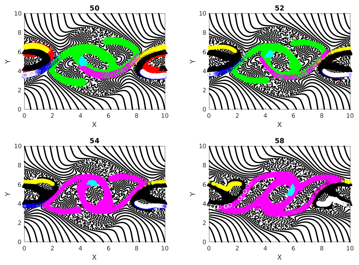
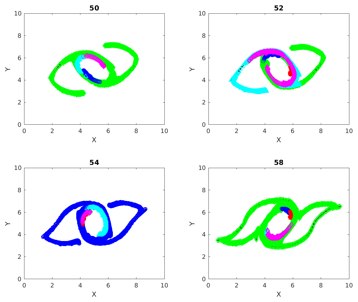
https://www.nonlin-processes-geophys.net/26/307/2019/npg-26-307-2019-f03

Figure 3Cumulative clusters identified at time 50 with threshold distance for interaction ϵ=40 % of initial separation of particles on uniform rectangular grid and their evolution tracked at later time steps (52, 54 and 58). Changing colors denote the merging of two clusters when particles from two clusters interact.

Download

3 Results

3.1 Cumulative clusters

Figure 3 shows the different cumulative clusters, found at time 50–58 in the simulation, in different colors. By this time the double jet has undergone instability, and coherent vortices, as well as vorticity filaments, are formed (Fig. 1). As explained earlier, cumulative clusters are formed by particle–particle interactions that occur up to a particular time. The threshold separation ϵ for interaction between two particles is 40 % of the grid spacing in this case. We can see in this figure how different clusters merge during their evolutions. An example for this is the transition from time 52 to 54 in Fig. 3, where the green and magenta clusters merge into one magenta cluster. Two clusters merge into one when a particle from one cluster interacts with a particle from another cluster. A question that follows is the following: can new clusters take the place of old clusters when they merge? The answer is yes; we can easily show the formation of new clusters having size of the same order. We create another figure, Fig. 4, which is identical to Fig. 3, except for the threshold interaction distance ϵ set to equal 20 % of the initial spatial grid spacing now. Comparing Figs. 3 and 4, we see that the clusters in the latter are smaller than those in the first. This is obvious because fewer particles interact with a threshold distance equal to 20 % of the grid spacing. In particular, particles in the clusters shown in Fig. 4 interact more strongly than those in Fig. 3, and hence the clusters do not evolve the same way in the two cases. Specifically the clusters in the smaller 20 % case do not change size or merge, and their paths are more or less periodically moving around the coherent vortex.

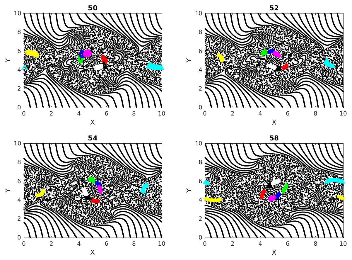
https://www.nonlin-processes-geophys.net/26/307/2019/npg-26-307-2019-f04

Figure 4Cumulative clusters found at time 50 with threshold distance for interaction ϵ=20 % of initial separation of particles on uniform rectangular grid and tracked at later time steps (52, 54 and 58). Changing colors denote the merging of two clusters when particles from two clusters interact.

Download

https://www.nonlin-processes-geophys.net/26/307/2019/npg-26-307-2019-f05

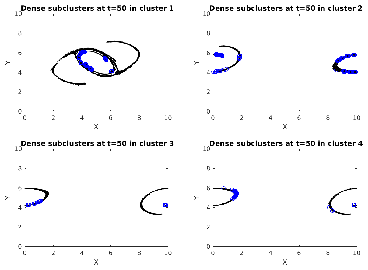
Figure 5Top four (1 being the largest) cumulative clusters (black) with their dense subclusters (blue) found at time 50. Spatially separated blue regions are distinct subclusters, with each of them having a minimum degree of 5 within themselves and hence being called dense.

Download

3.2 Dense subclusters

Figure 5 shows the four largest cumulative clusters with ϵ=40 % of the grid spacing, found at time 50 (particles in black), and also plots the dense subclusters mined from within these clusters (particles in blue). We number these clusters as cluster 1, 2, 3 and 4 in descending order of their sizes. Recalling the graph theoretic terminology from Sect. 2.3.1, we know that each of these subclusters is a graph with a minimum degree of 5. Dense subclusters locate the regions in a cluster where there are many interactions among particles significantly more than regions which are not blue. In simpler words these are places where particle interactions are at their peak. Particles in a dense cluster, if from sources with varying properties, are an example of localized mixing. Otherwise, if they are from the same source, the properties of that source remain preserved in that dense cluster. Mining γ quasi-cliques is thus useful for studying the traits of mixing specific to a problem. Interestingly, the blue regions in this figure have many similarities with the clusters in Fig. 4, which represents the stronger interactions. This tells us that the regions of stronger interactions are not very different from the regions of denser interactions in our double-jet flow. In Fig. 6, we show the local clustering coefficient and the node degree for the top four cumulative clusters at output time 50. Comparing with Fig. 5, it is not surprising to find that some particles from the dense subclusters have a large node degree and clustering coefficient, meaning that they have potential to form local clusters.

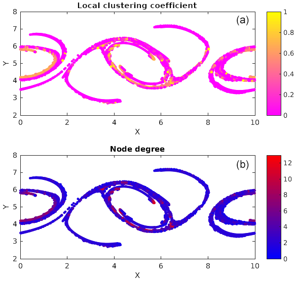
https://www.nonlin-processes-geophys.net/26/307/2019/npg-26-307-2019-f06

Figure 6Local clustering coefficient (a) and node degree (b) for the top four cumulative clusters at output time 50.

Download

Figures 7, 8 and 9 show the temporal evolution of cumulative clusters 1, 2 and 3 respectively and the temporal evolution of the particles in the dense-clusters. Figure 8 is different from Figs. 7 and 9 in the sense that some particles forming the dense subclusters in this figure appear to split from other particles in the dense subgroups. This means that particles from these regions of dense interactions move out of their more or less periodic paths and mix with particles in other regions of the flow. We measure the displacement of the particles in dense clusters within clusters 1, 2 and 3 from their positions at t=50 and plot them versus output times in Fig. 10. It is seen the paths are periodic with decreasing amplitude but have the same mean for clusters 1 and 2, meaning that the mean position of the particles slowly spirals toward the center of the vortex. For the second cluster, as mentioned earlier, the mean displacement increases, implying that some of the particles have escaped from their original vortex. In this particular case, this is an indication that these particles that have undergone dense and strong interactions have exchanged physical properties among themselves, and when they move out of their periodic paths to mix with outside particles in the flow, there is a chance that they transfer their properties in this foreign part of the flow by interaction.

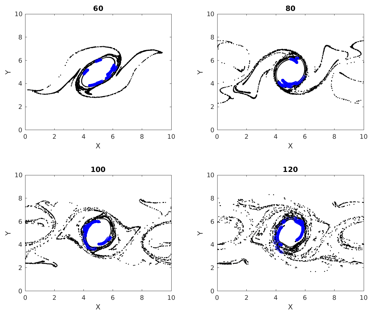
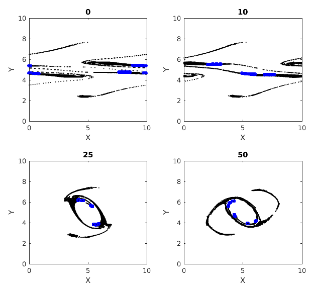
https://www.nonlin-processes-geophys.net/26/307/2019/npg-26-307-2019-f07

Figure 7Multiple time images of cumulative cluster 1 (black) with its dense subclusters (blue). Blue circles at later times represent particles that were parts of a dense subcluster at time 50.

Download

https://www.nonlin-processes-geophys.net/26/307/2019/npg-26-307-2019-f08

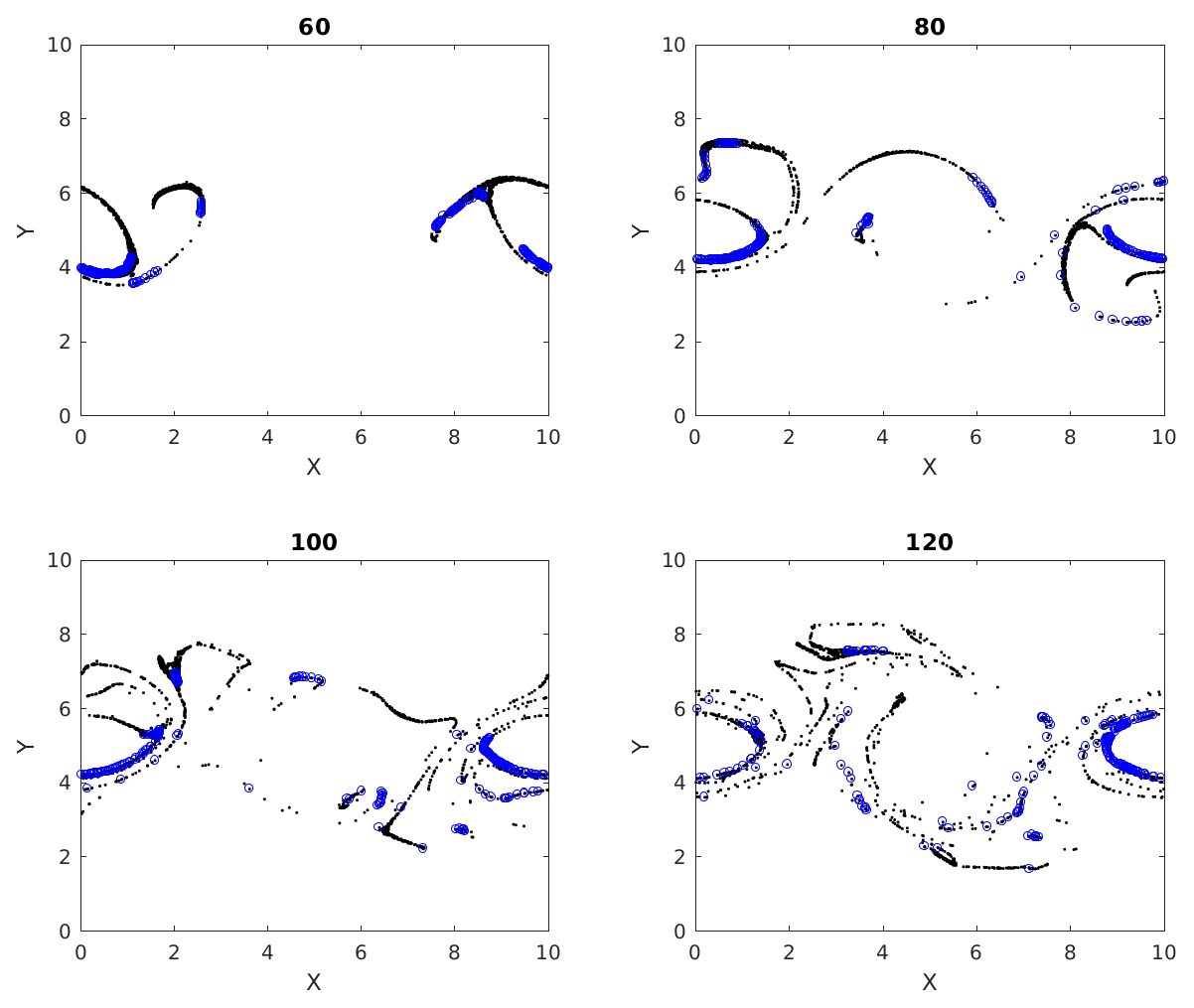
Figure 8Multiple time images of cumulative cluster 2 (black) with its dense subclusters (blue). Blue circles at later times represent particles that were parts of a dense subcluster at time 50.

Download

https://www.nonlin-processes-geophys.net/26/307/2019/npg-26-307-2019-f09

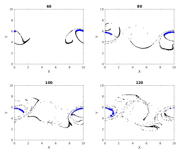
Figure 9Multiple time images of cumulative cluster 3 (black) with its dense subclusters (blue). Blue circles at later times represent particles that were parts of a dense subcluster at time 50.

Download

https://www.nonlin-processes-geophys.net/26/307/2019/npg-26-307-2019-f10

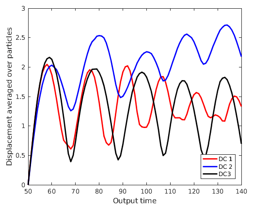
Figure 10Displacement averaged over particles in dense clusters from clusters 1, 2 and 3 (DC 1, DC 2 and DC 3) measured from positions at output time 50 vs. output time.

Download

3.3 Characteristics of dense subclusters

In this section we explore a few characteristics of the dense subclustering technique. The runtime of the Quick algorithm depends on the number of vertices V in the graph, the average degree d of the vertices, the minimum degree threshold γ, the size of quasi-cliques present and the number of quasi-cliques present. The data mining problem in this context does not have an a priori estimate. Hence the user has no control over the size and the number of quasi-cliques present. Liu and Wong (2008) study the effect of changing parameters on the runtime of the algorithm. The runtime, t_run, varies exponentially with respect to the parameters as $t_{run} \sim 10^{k_{v} V} 10^{k_{d} d} 10^{- k_{γ} γ}$ for some constants k_v, k_d and k_γ, depending on the graph.

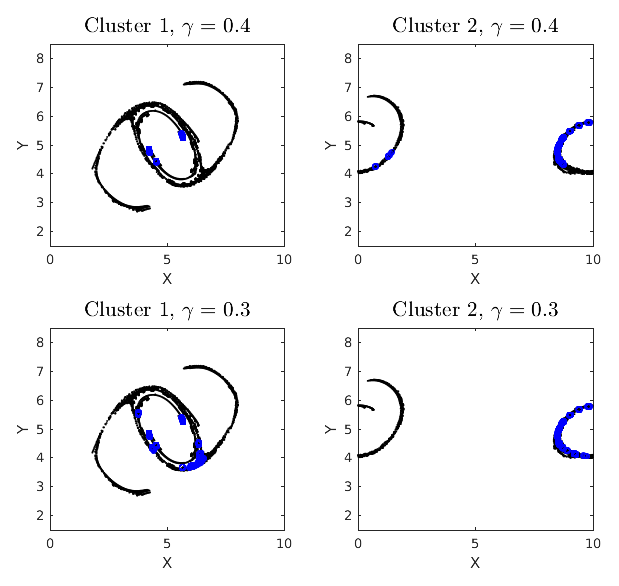
We wish to report the effects of changing ϵ and how to determine “the” ϵ for a problem. For the double-jet problem, increasing ϵ increases the size of the cumulative clusters considerably when compared at a fixed output time. An increase in the size of a cluster increases the computational complexity for Quick to mine the quasi-cliques exponentially. Let N be the total number of particles, and let C₄₀ and C₆₀ denote the particles in the biggest cumulative clusters for ϵ=40 % and ϵ=60 % respectively. Since N is fixed, C₄₀⊂C₆₀. To avoid excessive computational time and to draw comparisons on the same grounds, we look at the induced subgraph C₆₀[C₄₀]. The density of connections in C₆₀[C₄₀] is more than C₄₀; specifically, the average degree of nodes rises to 8.1 from 5.0. Again, to compare sets of the same class, we propose that $\frac{γ (min_size - 1)}{average_degree}$ is constant. Thus parameter min_size is kept constant , and γ is increased from 0.25 to 0.4. However, changing ϵ essentially changes the network, and the connections do not scale linearly. In Fig. 11, we look at dense clusters in cumulative clusters 1 and 2 with ϵ=60 %. The top left panel shows that the dense clusters mined with γ=0.4 and ϵ=60 % are a subset of those with γ=0.25 and ϵ=40 %. The remaining particles in the ϵ=60 % clusters cannot meet the tighter threshold criteria of the ϵ=40 % case. The bottom left panel shows the results with γ=0.3. Relaxing the minimum degree criteria yields more dense clusters, but some of them like those at the bottom of the vortex belong to a different class. This is because γ=0.3 does not scale properly with ϵ=60 %. This helps us understand the scenarios of increasing ϵ further, i.e., scaling up γ to make sure we remain consistent with our dense clusters. Otherwise, we are just mining densely connected graphs without physical meaning and taking a very long computational time to do so. The top and bottom right panels in the figure show the same results but for cumulative cluster 2 obtained with ϵ=60 %. It is interesting to observe in this case that improper scaling of γ might lead to repositioning of some of the maximal quasi-cliques; e.g., the dense cluster particles present in the left vortex of the γ=0.4 case are absent from the γ=0.3 case. This is because relaxing the threshold criteria caused the corresponding dense cluster to get bigger and exclude some of its previous residents. We also performed dense cluster analysis on ϵ=20 %, where the cumulative clusters are so small that almost all of them belong to the dense clusters. Hence, we suggest that the ideal ϵ be kept around half of the grid spacing and the ideal γ be kept as high as sufficient to obtain satisfactory quantity and quality of the dense clusters in a reasonable computational time. This requires some intuition on the part of the user but leads to the most robust results.

https://www.nonlin-processes-geophys.net/26/307/2019/npg-26-307-2019-f11

Figure 11Dense clusters with ϵ=60 % in cumulative clusters 1 and 2 at t=50.

Download

Increasing min_size would simply eliminate the dense clusters, which no longer meet the necessary criteria. However, it is important to note that it is necessary to tweak the min_size parameter for different cumulative clusters for best results. We show results of varying γ, keeping min_size constant in Fig. 12. Increasing γ beyond 0.4 does not yield any dense clusters in this case. The results themselves are quite intuitive and self-explanatory.

https://www.nonlin-processes-geophys.net/26/307/2019/npg-26-307-2019-f12

Figure 12Dense clusters with ϵ=40 % for varying γ at t=50.

Download

https://www.nonlin-processes-geophys.net/26/307/2019/npg-26-307-2019-f13

Figure 13Dense clusters with ϵ=40 % and particles on uniform rectangular grid.

Download

https://www.nonlin-processes-geophys.net/26/307/2019/npg-26-307-2019-f14

Figure 14Dense clusters with ϵ=40 % and particles on rectangular grid with perturbations.

Download

We tested the extent to which our dense clusters are sensitive to perturbations of initial particle distribution. Figure 13 shows the evolution of the dense clusters with uniformly distributed, random perturbations to the initial position of the particles. These had a maximum extent of 15 % of the grid spacing in each direction and ϵ=40 % in this case. The resulting dense clusters and their evolution are shown in Fig. 14. Comparing these two figures, we see that perturbing the particle positions changes the network and the location of the dense clusters, which is somewhat trivial. However, considering that this study is purely Lagrangian, the dense clusters from the perturbed case consistently convey qualitatively unchanged information about regions of potentially dense localized mixing (e.g., the ring of dense subclusters around the central vortex which can be traced backwards in time to the flanks of the geostrophically balanced jet).

https://www.nonlin-processes-geophys.net/26/307/2019/npg-26-307-2019-f15

Figure 15Spectral clusters found at multiple times from within cluster 1.

Download

3.4 Spectral clusters

In this section we show the results of spectral clustering described in Sect. 2.4. Figure 15 shows the different spectral subclusters that this algorithm splits the largest cumulative cluster (cluster 1) into. Figure 16 shows the temporal evolution of the spectral clusters of cluster 1 found at time 50. Giving a quick recap, the spectral clustering technique is responsible for dividing the set of particles into k communities, with k being 5 in the results shown. A spectral subcluster is expected to have more inter-particle interactions inside itself than outside because the clustering is applied on the adjacency matrix of particle interactions. The spectral subclusters are exhaustive, and hence unlike the dense subclusters, all of them are not equivalently rich in particles with high degrees of interaction. This can be seen from Fig. 16, where most of the particles in the subclusters of cluster 1 stay within the central vortex while some others take different paths over the course of the flow's evolution. This can be explained by our hypothesis that the paths of the densely interactive particles in cluster 1 tend to stay nearly periodic with time. Examining Fig. 15, we realize that the spatial distribution of these clusters shares similarities to some extent with the dense subclusters from the last subsection, especially around the coherent central vortex. This validates that these coherent structures are home to all the blue regions around the central vortex in Fig. 7, representing dense interactions and thereby strong mixing. Spectral clustering relies on k-means clustering and hence is highly sensitive to change in data distribution, e.g., different output times or small perturbations to initial particle distribution. Spectral clustering also returns subclusters of incomparable sizes, leaving us no way to compare the degree of mixing among the subclusters mined. The dense subclustering method, on the other hand, controls the density of connections and hence all subclusters mined belong to the same class of mixing.

https://www.nonlin-processes-geophys.net/26/307/2019/npg-26-307-2019-f16

Figure 16Spectral clusters in cluster 1 found at time 50 and tracked forward and backward.

Download

https://www.nonlin-processes-geophys.net/26/307/2019/npg-26-307-2019-f17

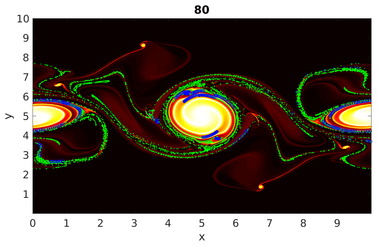
Figure 17Enstrophy field with particles at output time 80. The green dots represent particles from the three largest cumulative clusters, and the blue regions represent particles having dense interactions within these cumulative clusters.

Download

4 Conclusions

In this paper we have outlined a Lagrangian-particle-based technique to gain insight into mixing in non-linear geophysical flows. Our literature survey showed that clustering of particles based on inter-particle distances has been used to characterize mixing from a Lagrangian point of view. Local network measures like node degree and the local clustering coefficient of a particle, employed by previous researchers, e.g., Padberg-Gehle and Schneide (2017), gives an idea about the number of other particles that a chosen particle has interacted with, or “neighbors”. We have taken this approach one step further by finding subclusters representing regions of dense interactions. The findings of our work can be partly summarized by Fig. 17. In this figure we examine the output time 80, at which the double jet has broken up into a number of quasi-coherent vortices, as well as filaments of vorticity. The enstrophy field, scaled by its maximum, is shaded in the figure, with green dots superimposed to show particles from a few of the largest cumulative clusters. This gives us an indication of particles that have passed through regions where mixing has taken place. The algorithm Quick is used to identify subclusters of particles with dense mutual interactions (i.e., strongest mixing). These particles are plotted in blue. These particles, and their path history, identify regions where the degree of mixing is relatively higher (regulated by a density parameter γ) than other portions of the cumulative clusters. In summary, this figure tells us that the outskirts of the large, coherent vortices involve the strongest mixing. The vorticity filaments away from the quasi-coherent vortices are marked as belonging to regions of mixing but not the strongest mixing. The subclustering method thus provides a way to gain further detail on mixing intensity from a Lagrangian point of view.

We have compared our results with the coherent structures identified by spectral clustering. Spectral clustering shows that the location of the coherent structures is around the vortices but fails to point out the regions of strong mixing. As discussed in Sect. 2.4, the method of finding dense clusters is more precise and robust.

Summarizing the major findings in our work, we have seen that the size of cumulative clusters depends on the threshold interaction distance ϵ. In fact previous works like Padberg-Gehle and Schneide (2017) have only used values of ϵ larger than the grid spacing in order to make the entire graph connected and then apply techniques like spectral clustering to extract coherent sets. Our approach has allowed us to set ϵ to be smaller than the grid spacing (i.e., to demand stronger interactions as a proxy for more mixing) and observe the differences in cluster structure. We have inferred that cluster merging is possible beyond a threshold ϵ. Regions of strong and dense mixing are concentrated along the outskirts of the quasi-coherent vortices that develop spontaneously in the simulation, implying that coherent behavior can induce a lot of mixing, as demonstrated in Fig. 17. The highly interactive particles from the dense subclusters usually stay as a part of their original coherent vortex. However, interesting dynamics are present when some of these particles deviate out of their typical paths and mix with other regions in the flow, as discussed in Sect. 2.3. Indeed, results from spectral clustering show that some particles showing coherent behavior may become incoherent over time. The striking similarities between the behavior of the coherent spectral clusters and the dense subclusters indicate that dense interaction, and thereby inferred mixing, is a characteristic of coherent structures. A study of the effects of parameter variation on the dense subclustering technique showed that ϵ should be chosen small enough to produce a satisfactory amount of information content about the regions of mixing. The smaller the minimum degree of interaction, the stronger the mixing represented by the mined regions. The minimum degree is controlled by parameters min_size and γ, where min_size is really a choice of the user based on the application and γ can be tuned to hit the optimal minimum degree value. The technique thus requires some tuning from the user.

Future work divides into algorithmic improvements and applications. On the algorithmic side, we would like to automate the selection of search parameters (γ and min_size) in Quick, based on the adjacency matrix. A GPU-based implementation of the shallow-water-equation solver, the Lagrangian particle tracking and dynamic calculation of the inter-particle interactions will also be presented in a future paper. On the application side, the central future challenge is how to appropriately think of particles, and hence Lagrangian-based mixing ideas, in more complex models. For example, should particles migrate across isopycnal layer boundaries in multilayer models?

Data availability

The data we use for this work are simulation data, which are obtained by running code.

Author contributions

RC carried out majority of the computation, analysis and writing, including research and software development of clustering and data mining algorithms and parallelization of algorithms in CUDA. AC contributed to the software development of the numerical solver for shallow water equations in CUDA. MS carried out majority of the literature research and supervision of the work and also contributed to the editing of the paper.

Competing interests

The authors declare that they have no conflict of interest.

Review statement

This paper was edited by Harindra Joseph Fernando and reviewed by two anonymous referees.

References

Al-Kahby, H., Dannan, F., and Elaydi, S.: Non-standard discretization methods for some biological models. Applications of nonstandard finite difference schemes, World Scientific, Singapore, 155–180, 2000. a

Allshouse, M. R. and Peacock, T.: Lagrangian based methods for coherent structure detection, Chaos, 25, 097617, https://doi.org/10.1063/1.4922968, 2015. a

Ascher, U. M. and Petzold, L. R.: Computer methods for ordinary differential equations and differential-algebraic equations, SIAM, 61, 37–61, 1998. a

Davidson, P.: Turbulence: an introduction for scientists and engineers, Oxford University Press, North York, ON, Canada, 2015. a, b

Fiedler, M.: Algebraic connectivity of graphs, Czech. Math. J., 23, 298–305, 1973. a

Froyland, G.: An analytic framework for identifying finite-time coherent sets in time-dependent dynamical systems, Physica D, 250, 1–19, 2013. a

Froyland, G.: Dynamic isoperimetry and the geometry of Lagrangian coherent structures, Nonlinearity, 28, 3587, https://doi.org/10.1088/0951-7715/28/10/3587, 2015. a

Froyland, G. and Padberg-Gehle, K.: A rough-and-ready cluster-based approach for extracting finite-time coherent sets from sparse and incomplete trajectory data, Chaos, 25, 087406, https://doi.org/10.1063/1.4926372, 2015. a

Froyland, G., Santitissadeekorn, N., and Monahan, A.: Transport in time-dependent dynamical systems: Finite-time coherent sets, Chaos, 20, 043116, https://doi.org/10.1063/1.3502450, 2010. a

Hadjighasem, A., Karrasch, D., Teramoto, H., and Haller, G.: Spectral-clustering approach to Lagrangian vortex detection, Phys. Rev. E, 93, 063107, https://doi.org/10.1103/PhysRevE.93.063107, 2016. a, b

Hadjighasem, A., Farazmand, M., Blazevski, D., Froyland, G., and Haller, G.: A critical comparison of Lagrangian methods for coherent structure detection, Chaos, 27, 053104, https://doi.org/10.1063/1.4982720, 2017. a, b, c

Hussain, A. K. M. F.: Coherent structures–reality and myth, Phys. Fluids, 26, 2816, https://doi.org/10.1063/1.864048, 1983. a

Klimenko, A.: Lagrangian particles with mixing. I. Simulating scalar transport, Phys. Fluids, 21, 065101, https://doi.org/10.1063/1.3147925, 2009. a, b

Kline, S. J., Reynolds, W. C., Schraub, F., and Runstadler, P.: The structure of turbulent boundary layers, J. Fluid Mech., 30, 741–773, 1967. a

Kundu, P. K., Cohen, I., and Hu, H.: Fluid mechanics, Elsevier Academic Press, San Diego, 2004. a

Liu, G. and Wong, L.: Effective pruning techniques for mining quasi-cliques, in: Joint European conference on machine learning and knowledge discovery in databases, Springer, Springer, Berlin, Heidelberg, 33–49, 2008. a, b, c, d

Lloyd, S.: Least squares quantization in PCM, IEEE T. Inform. Theory, 28, 129–137, 1982. a

Mancho, A. M., Small, D., and Wiggins, S.: Computation of hyperbolic trajectories and their stable and unstable manifolds for oceanographic flows represented as data sets, Nonlin. Processes Geophys., 11, 17–33, https://doi.org/10.5194/npg-11-17-2004, 2004. a

Mendoza, C. and Mancho, A. M.: The Lagrangian description of aperiodic flows: a case study of the Kuroshio Current, arXiv preprint, arXiv:1006.3496, 2010. a

Garland, M., Le Grand, S., Nickolls, J., Anderson, J., Hardwick, J., Morton, S., Phillips, E., Zhang, Y., and Volkov, V.: Parallel computing experiences with CUDA, IEEE Micro, 28, 13–27, 2008. a

NVIDIA Corporation: CUDA CUFFT Library, version PG-05327-032_V02, NVIDIA Corporation, CA, USA, 2010. a

Padberg-Gehle, K. and Schneide, C.: Network-based study of Lagrangian transport and mixing, Nonlin. Processes Geophys., 24, 661–671, https://doi.org/10.5194/npg-24-661-2017, 2017. a, b, c, d, e, f

Prants, S.: Chaotic Lagrangian transport and mixing in the ocean, Eur. Phys. J.-Spec. Top., 223, 2723–2743, 2014. a

Rose, K. A., Fiechter, J., Curchitser, E. N., Hedstrom, K., Bernal, M., Creekmore, S., Haynie, A., Ito, S.-i., Lluch-Cota, S., Megrey, B. A., Edwards, C. A., Checkley, D., Koslow, T., McClatchie, S., Werner, F., MacCall, A., and Agostini, V.: Demonstration of a fully-coupled end-to-end model for small pelagic fish using sardine and anchovy in the California Current, Prog. Oceanogr., 138, 348–380, 2015. a

Rypina, I. I. and Pratt, L. J.: Trajectory encounter volume as a diagnostic of mixing potential in fluid flows, Nonlin. Processes Geophys., 24, 189–202, https://doi.org/10.5194/npg-24-189-2017, 2017. a

Salmon, R.: Lectures on geophysical fluid dynamics, Oxford University Press, North York, ON, Canada, 1998. a, b

Shi, J. and Malik, J.: Normalized cuts and image segmentation, Departmental Papers (CIS), p. 107, 2000. a

Zeng, Z., Wang, J., Zhou, L., and Karypis, G.: Coherent closed quasi-clique discovery from large dense graph databases, in: Proceedings of the 12th ACM SIGKDD international conference on Knowledge discovery and data mining, 20–23 August 2006, Philadelphia, PA, USA, ACM, 797–802, 2006. a

Articles