A prototype stochastic parameterization of regime behaviour in the stably stratified atmospheric boundary layer

Abraham, Carsten; Holdsworth, Amber M.; Monahan, Adam H.

doi:https://doi.org/10.5194/npg-26-401-2019

Articles | Volume 26, issue 4

https://doi.org/10.5194/npg-26-401-2019

Articles | Volume 26, issue 4

Research article

15 Nov 2019

Research article |

| 15 Nov 2019

A prototype stochastic parameterization of regime behaviour in the stably stratified atmospheric boundary layer

Carsten Abraham, Amber M. Holdsworth, and Adam H. Monahan

Abstract

Recent research has demonstrated that hidden Markov model (HMM) analysis is an effective tool to classify atmospheric observations of the stably stratified nocturnal boundary layer (SBL) into weakly stable (wSBL) and very stable (vSBL) regimes. Here we consider the development of explicitly stochastic representations of SBL regime dynamics. First, we analyze whether HMM-based SBL regime statistics (the occurrence of regime transitions, subsequent transitions after the first, and very persistent nights) can be accurately represented by “freely running” stationary Markov chains (FSMCs). Our results show that despite the HMM-estimated regime statistics being relatively insensitive to the HMM transition probabilities, these statistics cannot all simultaneously be captured by a FSMC. Furthermore, by construction a FSMC cannot capture the observed non-Markov regime duration distributions. Using the HMM classification of data into wSBL and vSBL regimes, state-dependent transition probabilities conditioned on the bulk Richardson number (Ri_B) or the stratification are investigated. We find that conditioning on stratification produces more robust results than conditioning on Ri_B. A prototype explicitly stochastic parameterization is developed based on stratification-dependent transition probabilities, in which turbulence pulses (representing intermittent turbulence events) are added during vSBL conditions. Experiments using an idealized single-column model demonstrate that such an approach can simulate realistic-looking SBL regime dynamics.

Download & links

Article (PDF, 7591 KB)

How to cite

How to cite.

Dates

Received: 29 Sep 2018 – Discussion started: 11 Oct 2018 – Revised: 08 Oct 2019 – Accepted: 10 Oct 2019 – Published: 15 Nov 2019

1 Introduction

A common classification scheme of the stably stratified atmospheric boundary layer (SBL) distinguishes between two distinct regimes, denoted the weakly and very stable boundary layers (respectively, wSBL and vSBL, e.g. Mahrt, 1998 a, 2014; Acevedo and Fitzjarrald, 2003; van Hooijdonk et al., 2015; Monahan et al., 2015; Vercauteren and Klein, 2015; Acevedo et al., 2016; Vignon et al., 2017 b; Abraham and Monahan, 2019 b, c, hereafter AM19a, AM19b, and AM19c). In this classification scheme the wSBL is characterized by weak stratification, strong wind, and shears which produce sufficient turbulence kinetic energy (TKE) to sustain continuous vertical mixing despite the stable stratification (e.g. van de Wiel et al., 2012). The vSBL is characterized by strong stratification, low wind speeds, and weak or intermittent turbulence such that vertical coupling of the atmospheric layers weakens. Very stable boundary layers are also sometimes found to display so-called upside-down turbulence, in which TKE is generated aloft by strong shears and then transported downwards. Observational data as well as simulations show that, to a good approximation in horizontally homogenous conditions, the wSBL conforms to the classical understanding of turbulence in the atmospheric boundary layer, with turbulence quantities decreasing with height and near-surface profiles which are well described by Monin–Obukhov similarity theory (MOST; e.g. Sorbjan, 1986; Mahrt, 1998 a, b, 2014; Pahlow et al., 2001; Grachev et al., 2005, 2013). In the vSBL, on the other hand, turbulence profiles can decouple from the surface (Banta et al., 2007) and MOST breaks down (e.g. Derbyshire, 1999; Banta et al., 2007; Williams et al., 2013; Mahrt, 2011; Optis et al., 2015). Regime structures and transitions are poorly represented in weather and climate models, due both to coarse resolution (vertical and horizontal) and to an imperfect understanding of the diverse physical processes governing the SBL, particularly with regard to the vSBL to wSBL transitions (e.g. Holtslag et al., 2013; Mahrt, 2014). In this study we first analyze how well the statistics of SBL regime occupation and regime transitions can be described by a two-regime system, with the goal of using this information to develop a prototype explicitly stochastic parameterization of turbulence in the SBL for models of weather and climate.

As transitions between the two SBL regimes are a common feature of SBL dynamics around the globe (AM19b), a representation of the effect of these dynamics in weather and climate models is needed. The regime transitions, however, are associated with a range of different mechanisms. Over land, the wSBL to vSBL transition (which for simplicity we denote the collapse of turbulence even though turbulence does not cease entirely) is normally caused by radiative cooling at the surface increasing the inversion strength and suppressing vertical turbulent fluxes of momentum and heat. This process is relatively well understood and has been examined using conceptual and idealized single-column models (van de Wiel et al., 2007, 2017; Holdsworth et al., 2016; Holdsworth and Monahan, 2019; Maroneze et al., 2019) or direct numerical simulations of stratified channel flows (Donda et al., 2015; van Hooijdonk et al., 2017) and atmospheric boundary layers (e.g. Flores and Riley, 2011; Ansorge and Mellado, 2014). Radiative cooling leads to very shallow boundary layers which are typically not resolved well in large-scale circulation models. Another mechanism for the wSBL to vSBL transition of particular importance over water is the advection of warm air aloft (AM19c), producing vSBL conditions which are not as shallow as those driven by radiative fluxes.

The vSBL to wSBL transition (which we denote the recovery of turbulence) is less well understood. Mechanisms by which turbulence recovers include the build-up of shear resulting in instabilities or an increase in cloud cover weakening the stratification by increasing the downwelling longwave radiation (AM19b). Another potential class of processes initiating these transitions is associated with intermittent turbulence events (e.g. Mahrt, 2014, and references within), which have been found to dominate the turbulent transport in vSBL conditions (Nappo, 1991; Coulter and Doran, 2002; Doran, 2004; Basu et al., 2006; Acevedo et al., 2006; Williams et al., 2013). Intermittent turbulence arises from a range of different phenomena, such as breaking gravity waves or solitary waves (Mauritsen and Svensson, 2007; Sun et al., 2012), density currents (Sun et al., 2002), microfronts (Mahrt, 2010), Kelvin–Helmholtz instabilities interacting with the turbulent mixing (Blumen et al., 2001; Newsom and Banta, 2003; Sun et al., 2012), or shear instabilities induced from internal wave propagation (Sun et al., 2004, 2015; Zilitinkevich et al., 2008). It has also been suggested from direct numerical simulations that intermittency can arise as an intrinsic mode of the non-linear equations in the absence of external perturbations of the mean flow (Ansorge and Mellado, 2014). Regardless of which process causes the recovery of turbulence, all phenomena are subgrid scale in state-of-the-art weather and climate models and are typically not included explicitly through process-based deterministic parameterizations.

Although processes in the SBL have been extensively studied, substantial errors of SBL representation persist in weather and climate models (Dethloff et al., 2001; Gerbig et al., 2008; Bechtold et al., 2008; Medeiros et al., 2011; Kyselý and Plavcová, 2012; Tastula et al., 2012; Bosveld et al., 2014; Sterk et al., 2013, 2015). Misrepresentation of the SBL includes unrealistic decoupling of the atmosphere from the surface (due to misrepresentations of TKE in the vSBL), resulting in runaway surface cooling (Mahrt, 1998 b; Walsh et al., 2008), underestimation of the wind turning with height within the boundary layer (Svensson and Holtslag, 2009), overestimation of the boundary layer height (Bosveld et al., 2014), underestimated low-level jet speed (Baas et al., 2009), and underestimation of near-surface wind speed and temperature gradients or their diurnal cycle (Edwards et al., 2011).

Accurate simulations of these near-surface properties is particularly important for global and regional weather forecasts of vertical temperature structures which control the formation of fog and frost (Walters et al., 2007; Holtslag et al., 2013). More accurate simulations of the SBL regime behaviour are also important for better representations of surface wind variability and wind extremes (He et al., 2010, 2012; Monahan et al., 2011); simulation and assessment of pollutant dispersal, air quality (Salmond and McKendry, 2005; Tomas et al., 2016), harvesting of wind energy (Storm and Basu, 2010; Zhou and Chow, 2012; Dörenkämper et al., 2015); and agricultural forecasts (Prabha et al., 2011; Holtslag et al., 2013).

Global and regional weather and climate models often use an artificially enhanced surface exchange under stable conditions in order to improve simulations of the large-scale flow (Holtslag et al., 2013). This approach led to the introduction of long-tailed stability functions and minimum background TKE values that are not supported by observations. In such representations, turbulence is artificially sustained under very stable conditions and the two-regime characteristic of the SBL is suppressed, biasing near-surface winds and temperature profiles. Without such parameterizations the nocturnal boundary layers can experience a single turbulence collapse which persists for the entire night. Although the long-tailed stability functions in relatively coarse-resolution models are designed to mimic the grid box mean of fluxes over many subgrid-scale wSBL and vSBL patches, with increasing horizontal and vertical resolution more accurate process-based parameterizations are necessary. The occurrence of vSBL to wSBL transitions does not appear to depend deterministically on internal or external state variables (AM19a,b), indicating that parameterizations of the effects of these kinds of transitions in weather and climate models may be required to be explicitly stochastic (e.g. He et al., 2012; Mahrt, 2014). In particular, phenomena such as intermittent turbulence events will likely rely on stochastic parameterizations as their structure and propagation are found to be only weakly dependent on mean states (e.g. Rees and Mobbs, 1988; Lang et al., 2018). Stochastic subgrid-scale parameterizations of SBL processes have been proposed to account for the missing variability in the SBL and improve both climate mean states and forecast ensemble spread (e.g. He et al., 2012; Mahrt, 2014; Nappo et al., 2014; Vercauteren and Klein, 2015). For instance, Vercauteren and Klein (2015) propose an additional Markovian system to switch between times of strong and weak influence of short-timescale, non-turbulent motions on TKE production in the vSBL.

In AM19a,b,c it was demonstrated that hidden Markov model (HMM) analysis of Reynolds-averaged mean states can be used as a tool to analyze the SBL regimes at tower sites in many different settings. Independent of the surface type, the climatological setting, or the complexity of the surrounding topography, two distinct regimes in the state variable spaces of Reynolds-averaged mean states and turbulence are evident. As the HMM analyses provide climatological (that is, based on long-term statistics) transition probability matrices for a two-regime Markovian system, a natural approach to developing stochastic parameterizations of SBL regime dynamics is to investigate whether these can be based on “freely running” stationary Markov chains (FSMCs) using these transition matrices. The first goal of this study is to determine whether climatological Markovian transition probability matrices, which are by construction independent of the state of the SBL, are adequate for simulations of the SBL regime dynamics. While the HMM analyses presented in AM19a assume stationary Markov regime dynamics, statistical analyses of the estimated regime sequences show clear evidence of elevated probability of turbulence collapse close to sunset (AM19b). Furthermore, probability distributions of event durations demonstrate a localized maximum corresponding to a typical recovery time of 1 to 2 h after transitions, during which a subsequent transition is unlikely. This structure is indicative of non-Markov behaviour (AM19b). Because of these non-stationary and non-Markov behaviours, a FSMC will never exactly capture all aspects of SBL regime dynamics. However, it is a parsimonious model and might be sufficient to reproduce most statistics of interest.

In order to investigate the potential of FSMC-based parameterizations, we first analyze how well they can characterize the HMM-based regime statistics. As part of this analysis we consider the sensitivity of the regime sequence estimated by the HMM to perturbations of the persistence probabilities, allowing for a quantification of which ranges of persistence probabilities accurately describe SBL regime statistics in HMM analyses. By comparing this sensitivity analysis with a sensitivity analysis of regime statistics to varying persistence probabilities in a FSMC, we quantify which ranges of persistence probabilities are consistent with both SBL regime statistics derived from an HMM analysis and SBL regime statistics simulated in a FSMC. As we demonstrate that FSMCs cannot adequately simulate all SBL regime statistics of interest, we then investigate the state dependence of observed SBL regime transition probabilities. Finally, we develop a pragmatic prototype of an explicitly stochastic parameterization using the derived state-dependent transition probabilities and present preliminary tests in an idealized single-column model (SCM; Holdsworth and Monahan, 2019). The study is organized as follows. First a short review of the observational data used in the HMM analysis is given in Sect. 2, followed by a brief review of the HMM application to the SBL (Sect. 3). Results of simulating statistics in FSMC are shown in Sect. 4, followed by the description of the prototype state-dependent stochastic parameterization and test simulations in Sect. 5. Conclusions follow in Sect. 6.

2 Data

Only a brief summary is presented here because the observational data used in this study have been discussed in detail in AM19a. Observational data sets from nine different research towers measuring standard Reynolds-averaged meteorological state variables with a time resolution of 30 min or finer are considered (Table 1). The observational levels of wind speeds and temperatures determine the reference state variable sets which are used in the HMM analyses to classify the data into SBL regimes (cf. AM19a, Table 1). Substantial differences among the nine experimental sites exist in terms of their surface conditions, surrounding topography, and meteorological setting. As a simple classification scheme, we distinguish between land-based, glacial-, and sea-based stations.

Kaimal and Gaynor (1983)Blumen (1984)Ulden and Wieringa (1996)Brümmer et al. (2012)Floors et al. (2014)Gryning et al. (2016)Kalthoff and Vogel (1992)Wenzel et al. (1997)Barthlott et al. (2003)Bowen et al. (2000)Rishel et al. (2003)Genthon et al. (2010, 2013)Vignon et al. (2017 a, b)Beeken et al. (2008)Fischer et al. (2012)Dörenkämper et al. (2015)Fischer et al. (2012)

Table 1Basic information about the different land-, glacial-, and sea-based tower sites (geographical coordinates, time resolution) and their individual reference HMM state variable inputs Y (wind speeds W_h and static stabilities ΔΘ with their observational levels h) and reference transition probability matrices (Q_ref) of HMM analyses estimated from Y. Starting regimes for the transition probability matrices are denoted with a star. Transition probability matrices at Hamburg, Los Alamos, and DomeC are transformed to a 10 min time resolution, so a direct comparison to other sites is possible. To retrieve original transition probability matrices at these sites, the 1∕10, 3∕2, and 3 matrix powers (respectively) must be taken.

Download Print Version | Download XLSX

The land-based stations can be further clustered into different subsets. Both the Cabauw and Hamburg towers lie in flat, humid, grassland areas, although the Hamburg tower is affected by the large metropolitan area of Hamburg. The Karlsruhe tower is located in the Rhine Valley, a rather hilly, forested area. The American sites, Boulder and Los Alamos, are located in relatively arid settings and are strongly affected by the surrounding topography of the Rocky Mountains.

The DomeC observatory, the single glacial-based station, is located in the interior of Antarctica and is influenced by completely different surface conditions, including high albedo and low roughness length.

The sea-based stations are the offshore research platforms Forschungsplattform in Nord- und Ostsee (FINO), located in the German North and Baltic seas. These sites are characterized by relatively homogeneous local surroundings and a large surface heat capacity. At the FINO towers nights with statically unstable conditions (defined as nights with two or more unstable datapoints in a night) are excluded as under these conditions wind speed measurements are unreliable (Westerhellweg and Neumann, 2012). Furthermore, at FINO-1 nights with primary wind directions between 280 and 340^∘ are excluded due to mast interference effects in the data. At the other stations such an exclusion is not necessary as three wind measurements with 120^∘ separation are taken at each level.

3 Brief summary of the hidden Markov model

We now present a brief overview of the HMM analysis with application to the SBL (Monahan et al., 2015, AM19a). An in-depth description of HMM analyses can be found in Rabiner (1989).

We use the HMM to systematically characterize regime behaviour in the SBL from observed data. The HMM assumes that underlying the observations is an unobserved, or hidden, discrete Markov chain ( $X = {x_{1}, x_{2}, \dots, x_{T}}$ ). The analysis estimates the regime-dependent parametric probability density distribution (pdf) of the observations (described by the parameter set λ), the transition probability matrix Q, and a most likely regime path of the Markov chain (known as the Viterbi path, VP). We associate the different states of the Markov chain with the SBL regimes (wSBL and vSBL). In our analysis we use observations of the three-dimensional vector consisting of the Reynolds-averaged vertically averaged mean wind speed, wind speed shear, and stratification to define the HMM input vector Y. A detailed justification of this observational input data set is presented in AM19a. The HMM estimation algorithm makes use of the following assumptions.

Markov assumption: the current regime value i_t at x_t depends exclusively on the previous regime of x_t−1, so
$\begin{matrix} (1) & \begin{aligned} P (x_{t} = i_{t} | x_{t - 1} = i_{t - 1}, x_{t - 2} = i_{t - 2}, \dots, x_{0} = i_{0}) \\ = Q_{i_{t} i_{t - 1}} \forall t with i \in {0, 1}, \end{aligned} \end{matrix}$
where the dynamics of the SBL are governed by Q (a 2×2 matrix corresponding to the wSBL and vSBL, respectively) such that $\sum_{i_{t}} Q_{i_{t} i_{t - 1}} = 1$ .
Independence assumption: conditioned on X, values of Y are independent and identically distributed variables resulting in a probability of the observational data sequence of
$\begin{matrix} (2) & \begin{aligned} P (Y, X | Λ) = π_{i} p (y_{0} | x_{0} = i_{0}, λ_{i_{0}}) \prod_{t = 1}^{T} Q_{i_{t} i_{t - 1}}, \\ p (y_{t} | x_{t} = i_{t}, λ_{i_{t}}) with i \in {0, 1}, \end{aligned} \end{matrix}$
where $Λ = {\{λ_{i}, π_{i}, Q\}}_{i \in {0, 1}}$ is the full set of parameters of the HMM, for which ${\{λ_{i}\}}_{i \in {0, 1}}$ is the parameter set describing the regime-dependent pdfs of y_t (taken to be Gaussian mixture models as in AM19a), and π_i is the probability that x₀ is in regime i (wSBL or vSBL).
Stationarity assumption: this analysis assumes that Q and ${λ_{i}}_{i \in {0, 1}}$ are time-independent.

The goal of the HMM analysis is to estimate Λ from Y. Starting from the probability of the observational time series conditioned on the parameters P(Y|Λ) and applying Bayes' theorem to obtain P(Λ|Y), the problem reduces to a maximum-likelihood estimation which can be iteratively solved to find local maxima via the expectation maximization algorithm (Dempster et al., 1979). Having estimated Λ, the most likely regime sequence (the VP) can be calculated. Regime occupation and transition statistics can then be obtained through analysis of the VP. The estimation of the parameters in the expectation-maximization scheme for our analysis is described in detail in Rabiner (1989).

One limitation of the HMM model considered is that it assumes stationary statistics. However, non-stationarities linked to the diurnal cycle and seasonal variability are present in the regime statistics of the SBL (cf. next section, AM19b). Generalizations exist which can account for non-stationarities, such as nonhomogeneous HMMs (Hughes et al., 1999; Fu et al., 2013) which condition transition probabilities on the state of external variables. Other clustering techniques such as the finite-element variational approaches also relax the stationarity assumptions (e.g. Franzke et al., 2009; Horenko, 2010; O'Kane et al., 2013). In particular, the finite-element, bounded-variation, vector autoregressive factor method (FEM-BV-VARX) includes both autoregressive dynamics within each regime and a modulation of regime dynamics to external drivers. For instance, Vercauteren and Klein (2015) were able to use this model to identify different regimes of interaction between submesoscale motions and the turbulence. However, as our analyses find no clear relationship between external drivers (geostrophic wind and cloud cover) and transitions between regimes of Reynolds-averaged variables (AM19b), we consider stationary HMM analysis in this study in order to investigate the simplest possible approach to a stochastic parameterization of turbulence under SBL conditions. Using such a relatively simple parameterization allows us to determine where additional complexity is warranted and assess how well the dynamics are approximated by stationary Markovian systems.

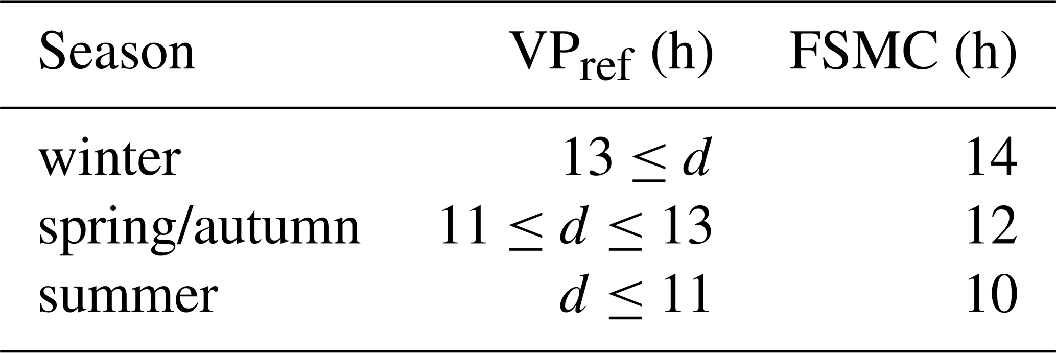
4 SBL regime statistics based on “freely running” Markov chains

To be useful as the basis of new parameterizations of turbulent fluxes in the SBL, FSMCs should model SBL regime statistics accurately. The statistics we focus on are the event durations and the probabilities of each of the occurrence of very persistent nights, of the occurrence of at least one transition within a night, and of multiple transitions within a night. Our reference FSMC models use transition matrices Q_ref obtained from HMM analyses in AM19a (Table 1). In the HMM analysis, the matrix Q can be held fixed at prescribed values while other parameters and the VP are estimated. Repeating HMM analyses using such fixed Q perturbed from Q_ref, we investigate the sensitivity of the regime statistics of corresponding VPs relative to their reference VP_ref. Because the estimated VP is constrained by the observations, its statistics may differ considerably from a FSMC using the same Q. Evaluating the FSMC regime statistics for a range of different Q determines the ranges of persistence probabilities for which SBL regime statistics of a FSMC match those of VP_ref. Mathematical expressions used to compute the regime statistics of a FSMC using a given Q are presented in Appendix A. These calculations require specification of the lengths of the nights. As the tower sites are located in the midlatitudes, we use a range of nighttime durations between 8 and 15 h. In this section we do not consider the glacial-based station, DomeC in Antarctica. Because the duration of the polar nights is much longer than nights at the other midlatitude stations considered, direct comparisons of regime occupation statistics within individual nights are not meaningful.

4.1 Comparison of VP_ref and FSMC statistics

For a FSMC (using Q_ref in Eqs. A1 and A2), the frequency of the occurrence of very persistent wSBL nights decreases monotonically with the length of the night (Fig. 1). Occurrence probabilities of very persistent wSBL nights from the FSMC match those of VP_ref in summertime (nights of duration 8 to 10 h), but are otherwise underestimated. For longer nights the FSMC underestimates their occurrence. The increase in occurrence probability with increasing night length in VP_ref is consistent with larger synoptic-scale variability and stronger mechanical generation of turbulence in winter, but is not accounted for in a FSMC. The occurrence probabilities of very persistent vSBL nights decrease with increasing length of night in VP_ref, consistent with an increase in mean pressure gradient force. While the FSMC also shows an increase, it systematically underestimates the observed occurrence of very persistent vSBL nights.

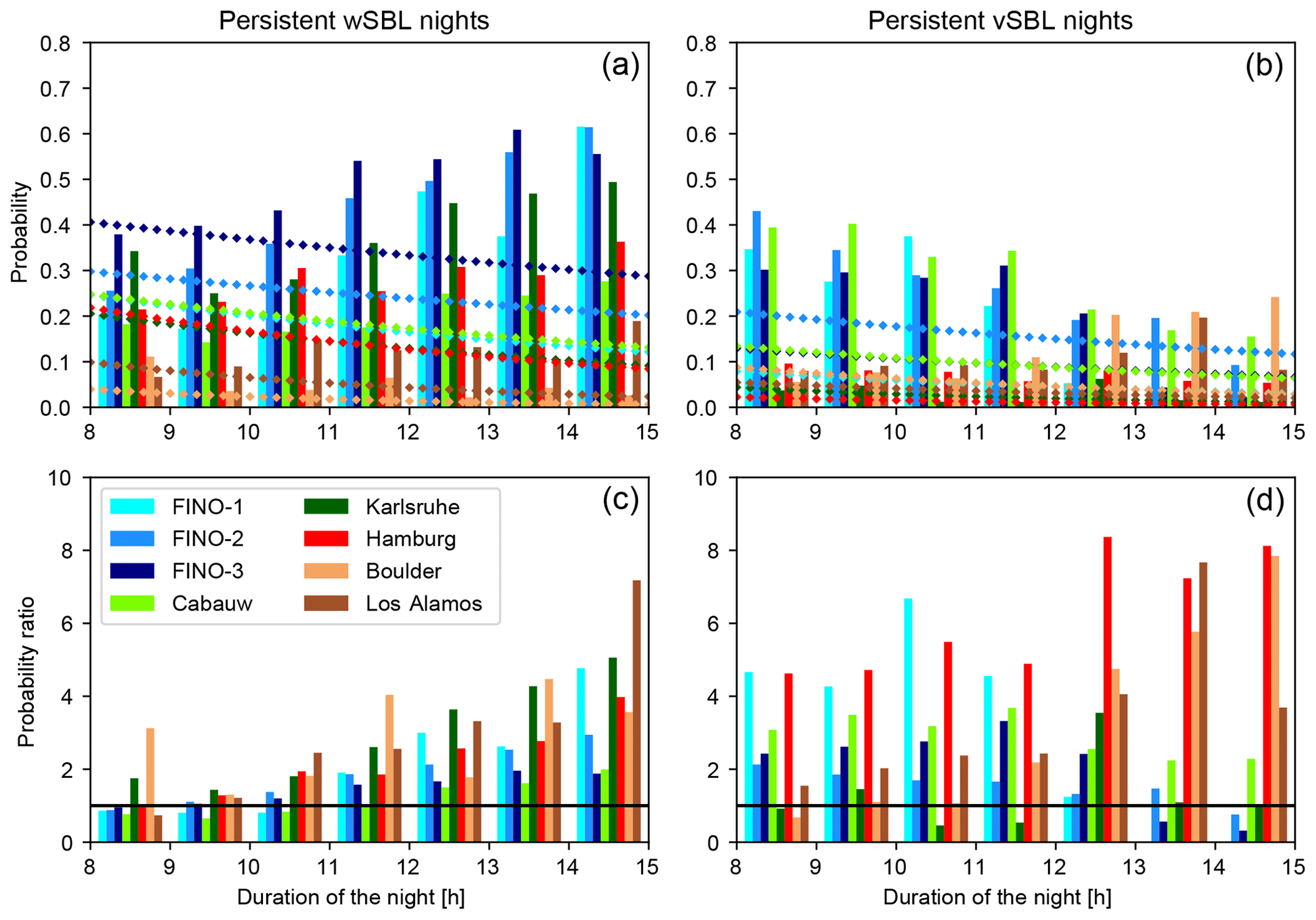
https://www.nonlin-processes-geophys.net/26/401/2019/npg-26-401-2019-f01

Figure 1Occurrence probabilities of very persistent wSBL (a, bars) and vSBL (b, bars) nights as estimated from VP_ref for nights of different lengths (in 1 h increments) at the different tower sites, compared to the occurrence probabilities of very persistent nights computed from the FSMC using Q_ref (diamonds). Lower panels show the ratio of the probabilities in the upper panels (values from the VP_ref divided by those from the FSMC).

Download

In VP_ref the probability of at least one wSBL to vSBL or vSBL to wSBL transition occurring within a night shows no systematic dependence on the length of the night across the tower sites (Fig. 2). In contrast, the occurrence probability of at least one transition in a FSMC (Eqs. A3 and A4) increases with the length of the night and is larger than the VP_ref at all sites (Fig. 2, lower panels). The overestimation of turbulence recovery events by the FSMC is slightly larger than that of turbulence collapse events at land-based stations, while the opposite is true at sea-based stations.

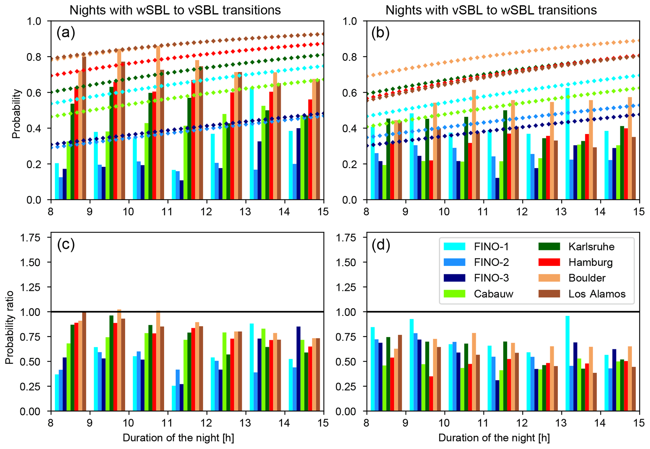
https://www.nonlin-processes-geophys.net/26/401/2019/npg-26-401-2019-f02

Figure 2As in Fig. 1 but for the occurrence probabilities of at least one wSBL to vSBL (a, c) or vSBL and wSBL (b, d) transition within a night.

Download

The probabilities of the occurrence of a recovery event subsequent to a turbulence collapse in the FSMC (Eqs. A6 and A8, Fig. 3) agree better with those of VP_ref than do the probabilities of the overall occurrence of at least one wSBL to vSBL transition (Fig. 2). Both VP_ref and FSMC occurrence probabilities increase with the length of the night, at about the same rate. At land-based stations the VP_ref has fewer subsequent turbulence recovery events than expected from a FSMC, and at sea-based sites more are observed than predicted by a FSMC. Distributions of wSBL to vSBL transitions subsequent to recovery events in a FSMC and the VP_ref are generally similar, with slightly better agreement in summer than winter (Fig. 3, right panels).

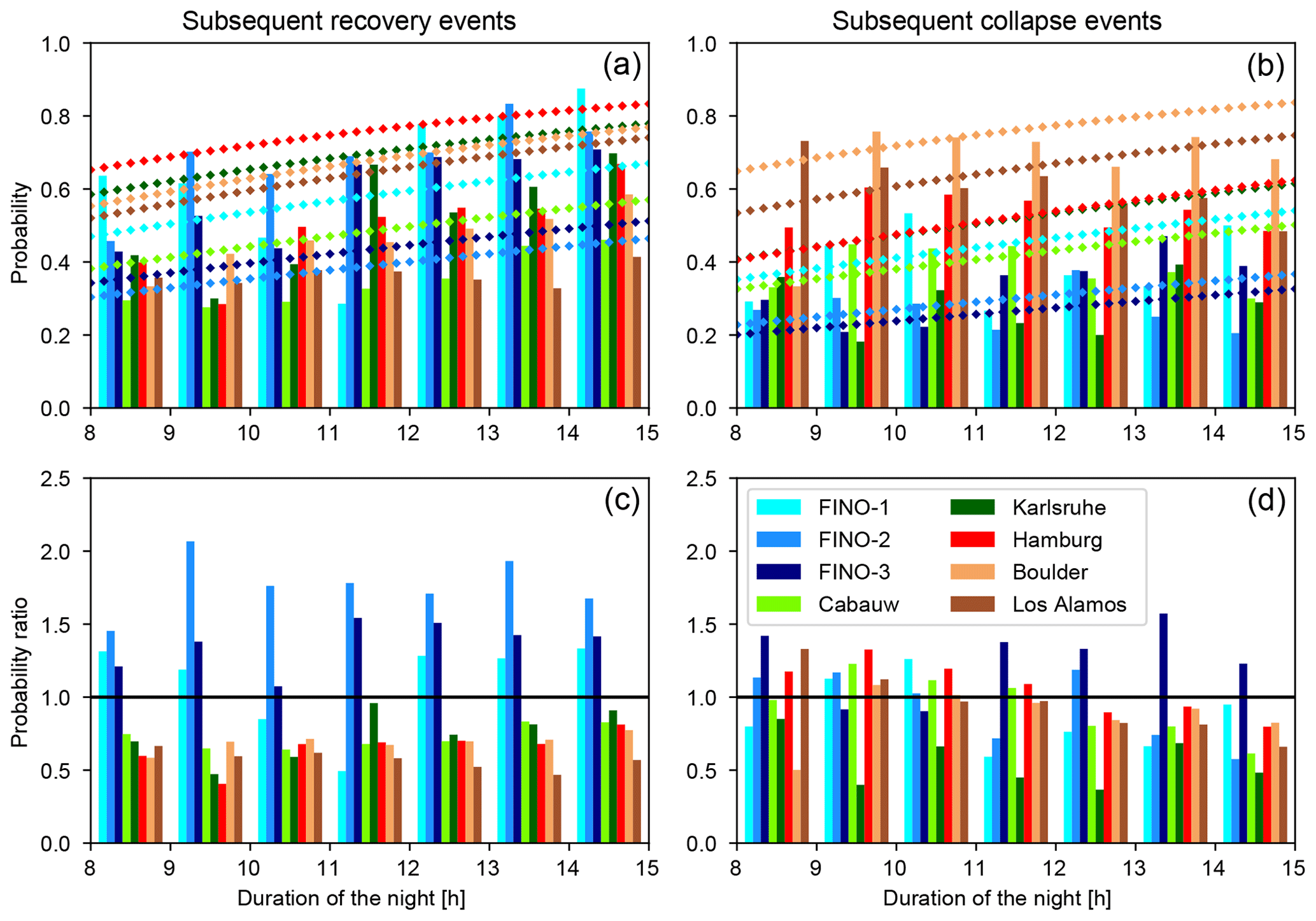
https://www.nonlin-processes-geophys.net/26/401/2019/npg-26-401-2019-f03

Figure 3As in Fig. 1 but for the probabilities of the occurrence of turbulence recovery events subsequent to turbulence collapse (a, c) and turbulence collapse events subsequent to turbulence recovery events (b, d).

Download

The occurrence of subsequent transition events is related to event durations in the vSBL and wSBL. For both types of events, the duration pdfs display clear maxima between 1 and 2 h after preceding transitions, demonstrating that the occurrence of subsequent transitions most often occurs after some recovery period (Fig. 4). No two-regime FSMC can account for these recovery periods because event duration pdfs in the FSMC always decay monotonically (Eqs. A5 and A7). After the initial recovery period, however, event duration pdfs are generally close in the VP_ref and FSMC (for a 12 h night duration), resulting in a generally good agreement of mean event durations. The qualitative shape of the event duration pdfs is insensitive to season, although during winter the probabilities of longer events increase (longer nights allow more time for longer events to occur). Consistently, different nighttime durations in the FSMC change the pdf decay rate (steeper and shallower for, respectively, shorter and longer nights); however, the substantial differences to pdfs estimated from VP_ref remain.

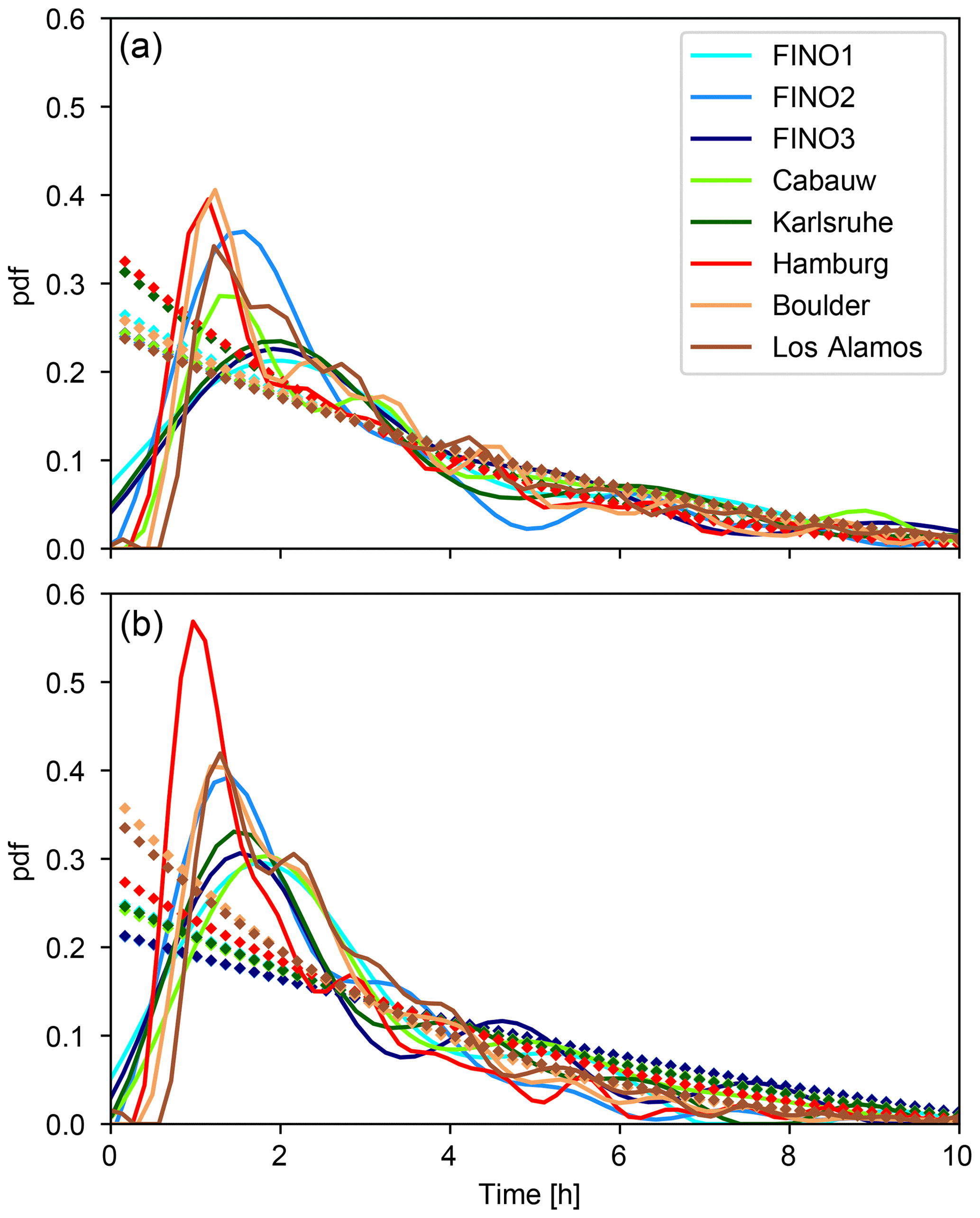
https://www.nonlin-processes-geophys.net/26/401/2019/npg-26-401-2019-f04

Figure 4Probability density functions of the vSBL (a) and wSBL event durations (b) as estimated from the VP_ref (solid lines) at the different tower sites compared to FSMC pdfs computed using Q_ref and a nighttime duration of 12 h (diamonds). All pdfs are calculated with the multivariate kernel density estimation by O'Brien et al. (2014, 2016).

Download

The results above demonstrate the existence of at least two aspects of the regime statistics which qualitatively cannot be accounted for by a two-regime FSMC: non-stationary and non-Markov behaviour. While many other regime statistics follow qualitatively the behaviour of a FSMC, quantitative differences between the statistics of VP_ref and FSMCs using Q_ref are substantial. As values on the diagonal of Q_ref are close to one (Table 1), the theoretical regime statistics calculated from the FSMC are highly sensitive to these values (cf. Eqs. A1–A8). Therefore, we now investigate the sensitivity of VP to perturbed Q to determine whether biases in the SBL regime statistics of the FSMC can be reduced by modest changes in Q.

4.2 Sensitivity of the VP to perturbed persistence probabilities

We consider the sensitivity of the VPs to changes in the persistence probabilities (diagonal elements of $Q_{i_{t} i_{t - 1}} = P (i_{t - 1} \to i_{t})$ with $i_{t} = i_{t - 1}$ and i∈{wSBL,vSBL}) by perturbing Q from the reference value, holding it fixed, and repeating the HMM analysis. In order to assess whether the perturbed VPs are consistent with VP_ref, we consider first the occupation consistency between the two (the fraction of time in which both VPs are in the same regime). As in AM19a, we then assess the consistency of the timing of transitions (simultaneity of transitions in the reference and perturbed VPs) as well as the representation of very persistent nights. These various metrics are then combined to obtain the total VP consistency. For this part of the analysis, we focus on the Cabauw tower data as we have analyzed these data extensively in AM19a. The same qualitative results are found using all the tower station data we have considered (not shown).

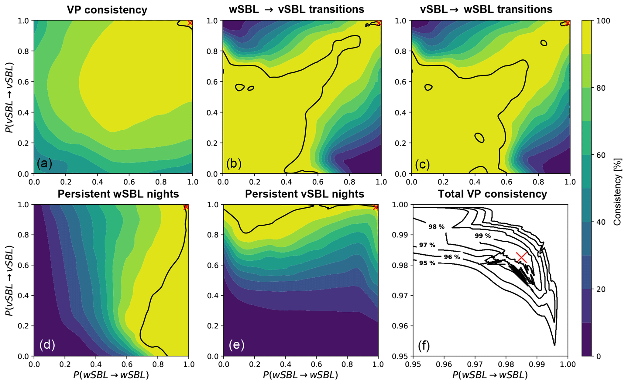
https://www.nonlin-processes-geophys.net/26/401/2019/npg-26-401-2019-f05

Figure 5Consistency of reference and perturbed regime occupation statistics as functions of Markov chain persistence probabilities at Cabauw. Displayed are the occupation consistency of the VP (a), the consistency of wSBL to vSBL (b) and vSBL to wSBL (c) transitions in the VP, and the consistency of the occurrence of very persistent wSBL (d) and vSBL (e) nights. The 99 % consistency values in each of these subpanels is delineated by a black line. Isolines of the total consistency of the perturbed and reference VP (ranges of persistence probabilities where all SBL regime statistics considered have the same or higher consistencies with VP_ref) are illustrated in panel (f). In each panel the reference value at Cabauw is shown by a red cross.

Download

The estimated VP is robust to substantial changes in Q, with an occupation consistency of more than 90 % obtained for ranges of wSBL and vSBL persistence probabilities between 0.5 and about 0.9999 (Fig. 5). Agreement at the 99 % level is found for persistence probabilities between approximately 0.9 and 0.9999. Accurate representation of the timing of transitions is found for both a broad range of low persistence probabilities and for a small range of persistence probabilities between 0.96 and 0.99. The fact that the accuracy of the transitions is above 99 % if both persistence probabilities are below 0.5 (regime transitions in a single step are more probable than remaining in the regime) is a consequence of the high frequency of modelled transitions improving the ability to capture individual transitions in VP_ref (at the expense of modelling far too many transition events). Because regime transitions are relatively rare, the physically meaningful range of persistence probabilities corresponds to relatively large values of both. The accuracy of the occurrence of very persistent wSBL nights in the perturbed VP is best for high P(wSBL→wSBL) and is weakly sensitive to P(vSBL→vSBL). This result is not surprising as the high wSBL persistence probability ensures that the majority of very persistent wSBL nights as estimated by VP_ref are captured. This measure is unaffected by any underestimate of the occurrence of very persistent vSBL nights. Complementary results are found for the occurrence of very persistent vSBL nights.

Each of the five consistency measures discussed captures distinct aspects of agreement between the reference and perturbed VPs. We define total consistency relative to VP_ref as each of the five described VP consistencies exceeding a specific threshold. At Cabauw, a 99 % total consistency can be achieved for P(wSBL→wSBL) between approximately 0.97 and 0.99 and P(vSBL→vSBL) between 0.98 and 0.99 (Fig. 5f). If only a 95 % total VP consistency is required, P(wSBL→wSBL) and P(vSBL→vSBL) can range approximately between 0.95 and almost 1.

The sensitivity analysis of the estimated regime occupation sequence to changes in Q values reveals that reasonably accurate HMM regime statistics can be obtained over a relatively large range of persistence probabilities. We now return to FSMC calculations using the ranges of Q where the total VP consistency exceeds 95 % to assess whether a common range of persistence probabilities exists where statistics of VP_ref and FSMC are consistent.

4.3 Sensitivity of SBL regime statistics to changing persistence probabilities in a FSMC

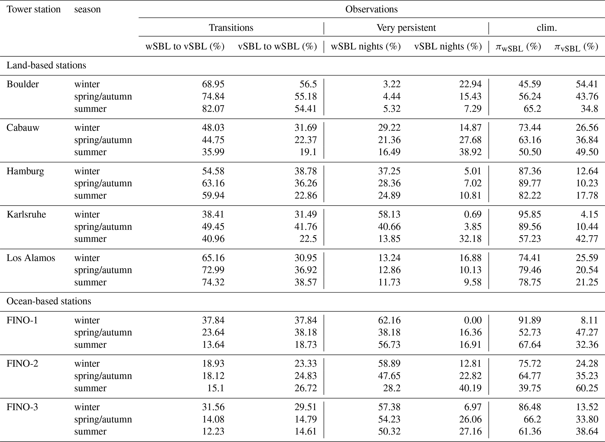
As discussed above, calculations of the theoretical values of SBL regime statistics from a FSMC require one to specify the duration of the night. To compare statistics from VP_ref and FSMC, we define three night durations representative of individual seasons (Table 2). The statistics from VP_ref for the individual towers and seasons are listed in Table 3. To account for sampling uncertainty in the SBL regime statistics as estimated from VP_ref, we consider occurrence probabilities in a 10 % error range (±5 %) around the values from VP_ref.

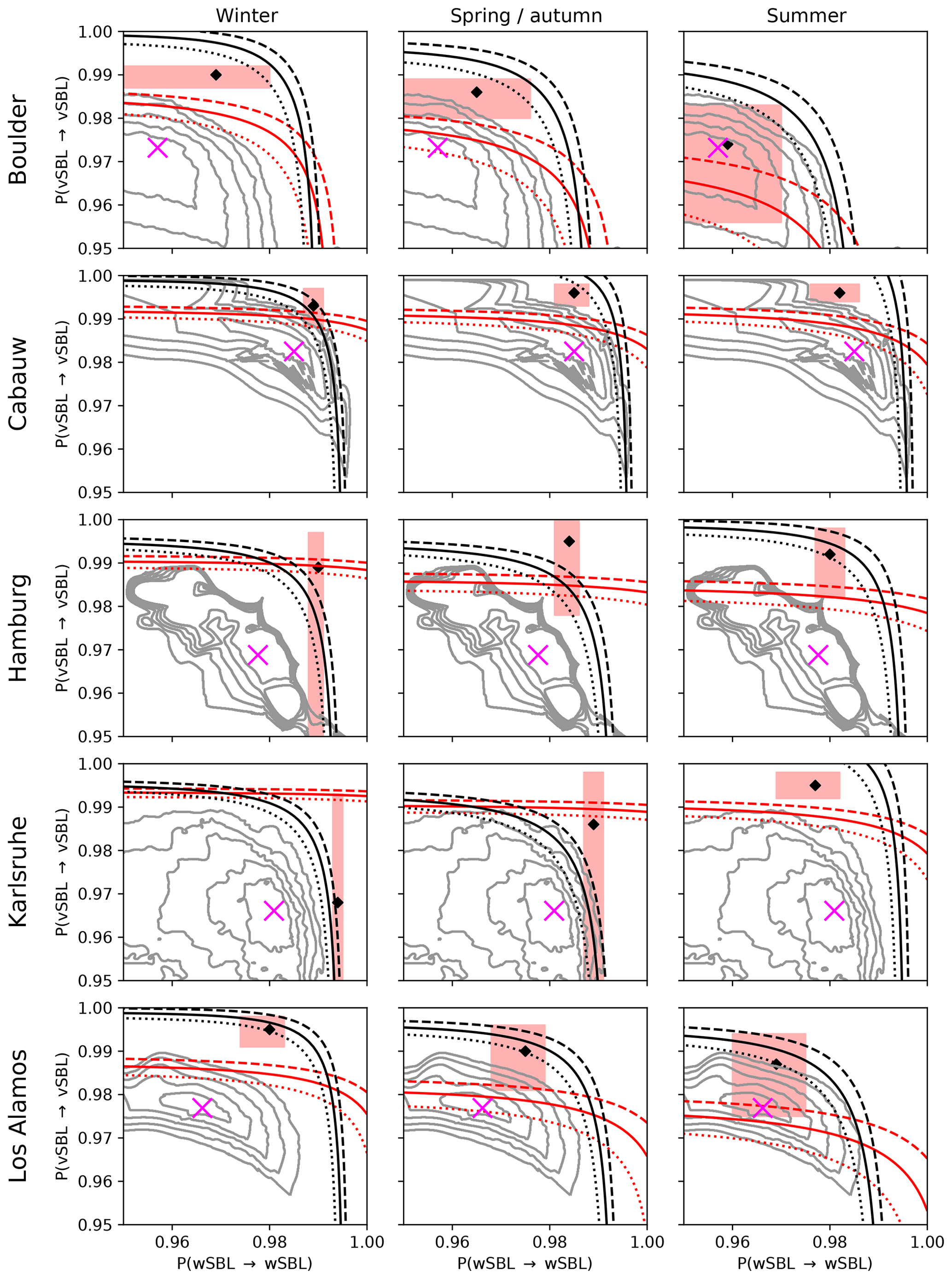
https://www.nonlin-processes-geophys.net/26/401/2019/npg-26-401-2019-f06

Figure 6Values of persistence probabilities for which the occurrence probability of at least one wSBL to vBSL transition in a night (red lines) or one vSBL to wSBL transition in a night (black lines) as computed from a stationary Markov chain equals the observed values. Solid, dashed, and dotted lines correspond to, respectively, the observed values, a probability of 5 % below the observed values, and a probability of 5 % above the observed values. The ranges of persistence probabilities where the occurrence probability of very persistent nights in a stationary Markov chain agrees with observations in a ±5 % uncertainty band is depicted by the red rectangle with a diamond displaying the values from VP_ref. The persistence probability values corresponding to 95 % to 99 % total consistency of the perturbed VP with VP_ref in the HMM analysis are depicted in grey contours. The persistence probabilities corresponding to Q_ref values are marked by a pink cross.

Download

Similar to what was found at Cabauw, across all land-based stations the perturbed VP is not very sensitive to the values of Q, and a relatively broad range of persistence probabilities allows for a 95 % total VP consistency in the HMM analyses (Fig. 6; grey isolines). The persistence probabilities corresponding to the most likely VPs are reasonably similar across the different stations. In Fig. 6 the solid, dashed, and dotted lines correspond, respectively, to persistence probabilities resulting in FSMC probabilities of at least one transition in a night equal to 5 % below and 5 % above the VP_ref values (wSBL to vSBL in red; vSBL to wSBL in black). The range of persistence probabilities for which the FSMC produces occurrence probabilities of very persistent nights within a 10 % uncertainty band around that of VP_ref is displayed by a red shaded rectangle with a mark for the exact VP_ref statistics.

Table 2Nighttime durations (d) for the different seasons for estimations of regime statistics from the VP_ref and corresponding average durations for calculations in a FSMC.

Download Print Version | Download XLSX

Despite accounting for non-stationarity by considering nights of different lengths separately, in general no ranges of persistence probabilities in any season can be identified for which FSMCs are able to model all SBL regime statistics within our imposed uncertainty range. Only at Cabauw in wintertime and Hamburg in spring or autumn does such a range of persistence probabilities exist.

In order to model only a subset of SBL regime statistics (such as the occurrence of SBL regime transitions or very persistent nights) accurately in a FSMC, the required persistence probability values generally fall outside the region of high total VP consistency between the reference and perturbed VPs. This fact is true for all seasons.

Table 3Probabilities of the occurrence probabilities of at least one wSBL to vSBL or vSBL to wSBL transition in a night, of the occurrence probabilities of very persistent wSBL or vSBL nights, and of the climatological initial distributions of starting a night in the wSBL or vSBL (or π_wSBL and π_vSBL) at the different tower sites for different seasons as estimated from the VP_ref.

Download Print Version | Download XLSX

At sea-based stations the range of persistence probabilities that ensures good agreement between the VP_ref and the perturbed VPs is substantially larger than for land-based stations (not shown). The total VP consistency exceeds 95 % for regime persistence probabilities ranging from approximately 0.92 to 0.99. Nonetheless, similar to land-based stations, no persistence probability range can be identified, which allows a FSMC to simulate all SBL regime statistics accurately. Again, to obtain only specific SBL regime statistics, ranges of persistence probabilities are required which generally exceed the values ensuring good agreement between the reference and perturbed VPs.

The fact that a FSMC is not able to account for all regime statistics (with or without seasonally varying Q) motivates the consideration of other approaches to the parameterization of regime dynamics. In particular, the use of state-dependent transition probabilities is supported by the relatively well-understood control of the internal SBL dynamics on wSBL to vSBL transitions (e.g. Acevedo et al., 2019; Maroneze et al., 2019, AM19b, AM19c), including the role of surface energy coupling (van de Wiel et al., 2017; Holdsworth and Monahan, 2019). In the next section we present a prototype of such a parameterization.

5 Stochastic parameterization for SBL regime dynamics

In this section, we develop a prototype explicitly stochastic parameterization for numerical weather prediction and climate models and test it using an idealized SCM. We first consider the state dependence of transition probabilities from VP_ref, to be used as the basis of a two-value (wSBL or vSBL) discrete SBL regime occupation variable (S). After having estimated functional forms for these conditional probabilities from fits to data, a parameterization of episodic enhancement of eddy diffusivity by intermittent turbulence bursts is developed. Finally, the application of this parameterization in the SCM is presented. We emphasize the fact that the explicitly stochastic parameterization and the tests of it presented here are intended to be a proof of concept. A formal validation of model experiments against observational data, including systematic sensitivity analyses of the free parameters and an implementation in a more complex single-column model, will be the subject of a future study.

5.1 State-dependent transition probabilities

The Richardson number (Ri) is often used in parameterizations of stratified boundary layer turbulence, and as such is a natural candidate on which to condition probabilities of transitions between states of S. For instance, we expect physically that $P (wSBL \to vSBL | R i)$ should be small for small Ri but should increase to virtual certainty for sufficiently large Ri.

Due to their coarse vertical sampling, the Reynolds-averaged observational tower data considered only allow for a characterization of finite-differenced approximations to Ri, in particular the bulk Richardson number (Ri_B):

\begin{matrix} (3) & R i_{B} = \frac{g}{\overline{Θ}} (h - s) \frac{Θ_{h} - Θ_{s}}{W_{h} - W_{s}}, \end{matrix}

where g is the acceleration due to gravity, $\overline{Θ}$ the mean background potential temperature, h the height of the upper measurement and s the lower measurement height near the surface, and Θ and W, respectively, the potential temperature and wind speed (at heights indicated by subscripts).

To assess the relationship between Ri_B and transition probabilities (and in particular the robustness of this relationship across different locations) we first investigate composites of its evolution during regime transitions at the various tower sites described in Sect. 2. These composites, centred on the time of transitions and extending 90 min before and after, characterize the average behaviour of Ri_B across transitions. Such composites do not distinguish differences between individual events which may be important for a detailed physical understanding of a specific transition. Furthermore, composite changes may be less sharp than individual ones, due to variations in transition timing below the averaging scale of the data considered.

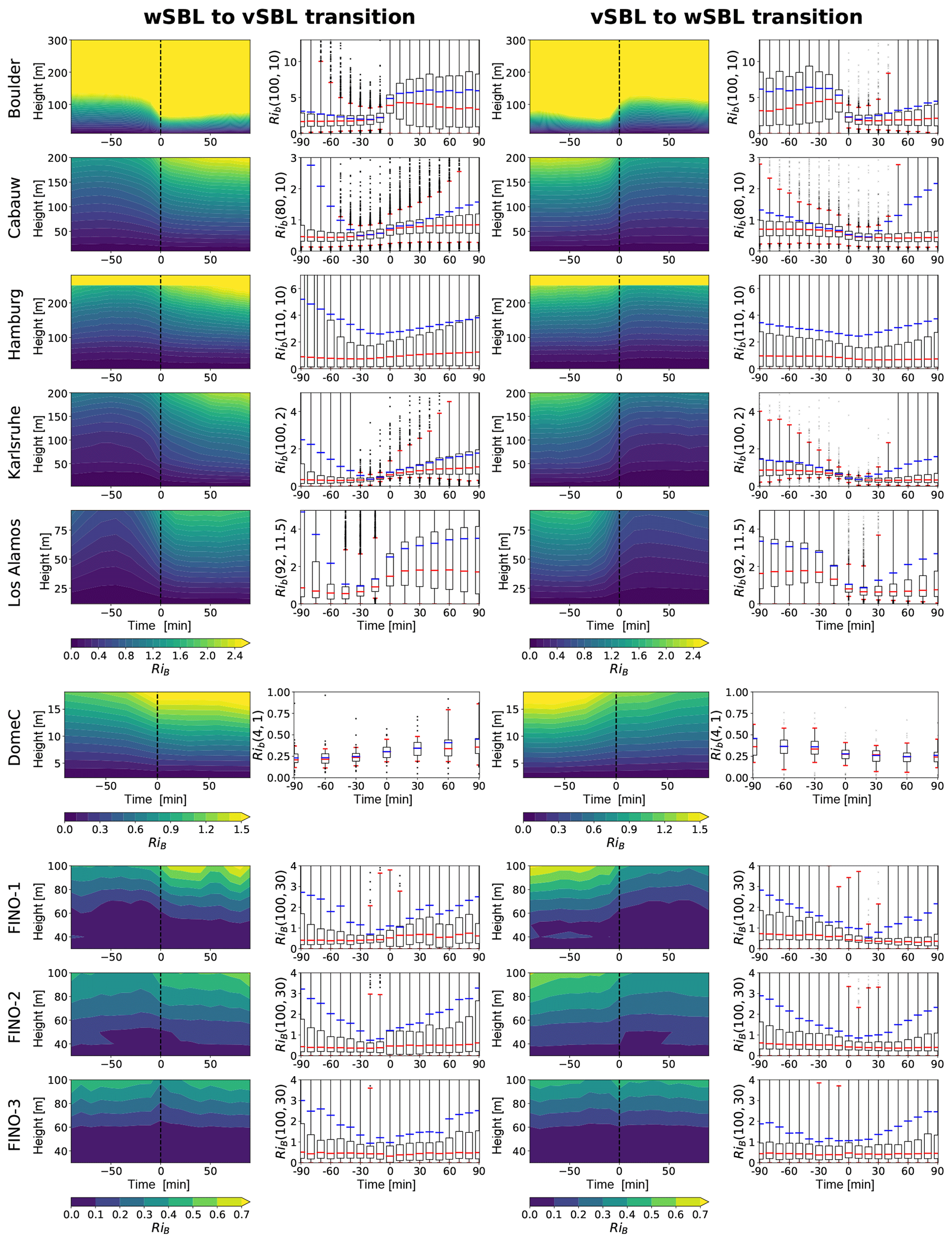
https://www.nonlin-processes-geophys.net/26/401/2019/npg-26-401-2019-f07

Figure 7Time evolution of the composite median of the bulk Richardson number (Ri_B; as determined between each observational level and about 10, 1, and 30 m for, respectively, the land-, glacial-, and sea-based tower stations) at the different tower sites in times of turbulence collapse (wSBL to vSBL transition; first and second columns) and turbulence recovery events (vSBL to wSBL transition; third and fourth columns) as determined by the HMM analyses. The composites show the 90 min before and after the transitions at time 0 (dashed reference line). Second and fourth rows: the distribution of the Ri_B showing the interquartile range (box), 5th to 95th percentile range (outer red bars), median, and mean values (or red and blue lines).

Download

Across all land- and glacial-based stations Ri_B measured between each observational height and the surface systematically increases (decreases) during turbulence collapse (recovery) events (Fig. 7, columns one and three). At sea-based sites changes in Ri_B are not evident. The weak signal in Ri_B at sea-based stations is likely related to the fact that the lowest observational levels are much farther from the surface than at other stations (30 m above mean sea level).

In order to further compare results across all tower sites, we concentrate on Ri_B between about 100 and 10 m (Ri_B(100,10)) for land-based stations. Because of the very shallow inversion at this location, at DomeC we use Ri_B between 4 and 1 m (cf. AM19c). The distributions of Ri_B(100,10) show that not only do the mean and median show a systematic behaviour across regime transitions, but so too does the interquartile range (Fig. 7, columns two and four). Consistent with previous results the distributions at sea-based stations do not change across transitions.

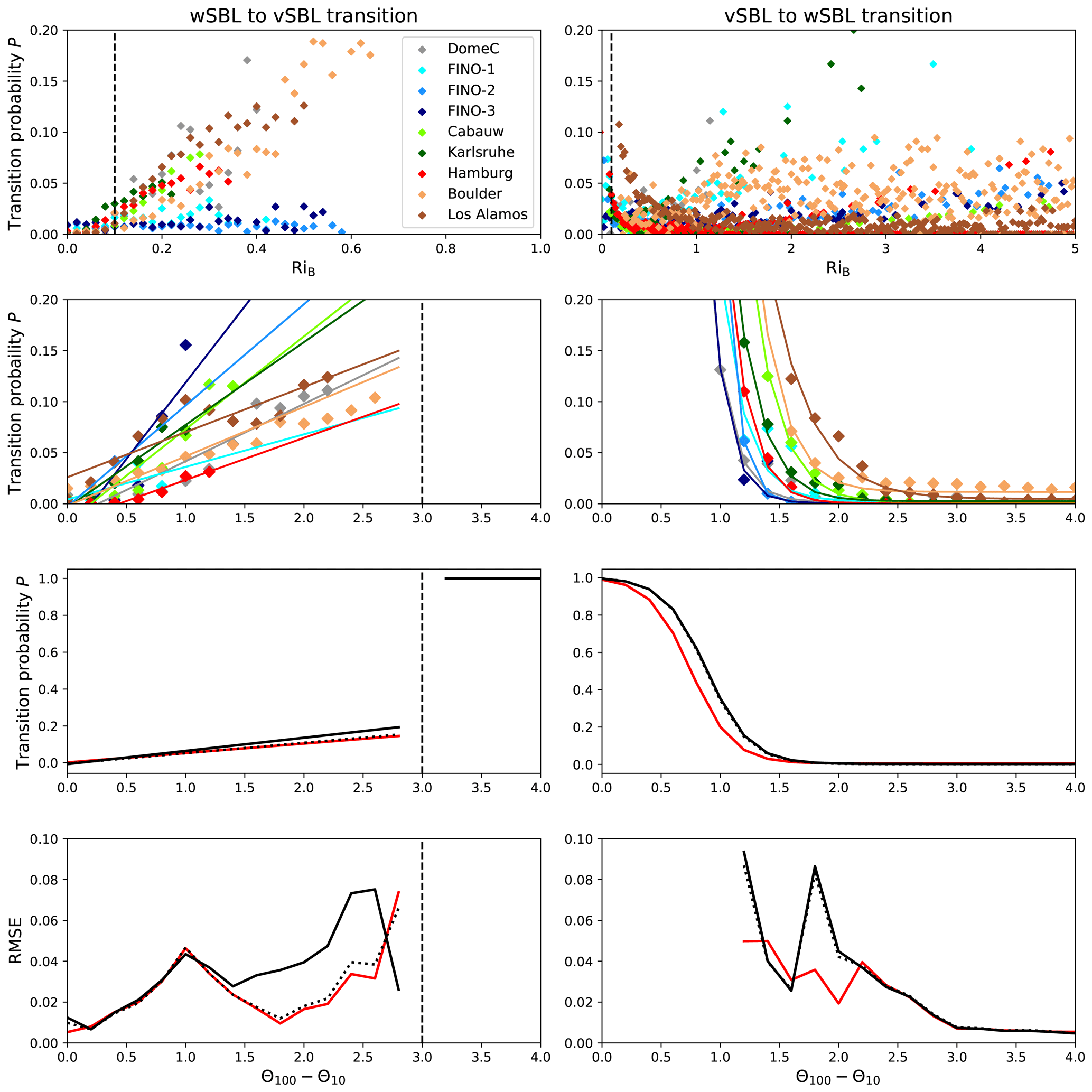
https://www.nonlin-processes-geophys.net/26/401/2019/npg-26-401-2019-f08

Figure 8First row: probabilities for wSBL to vSBL (left) and vSBL to wSBL transitions (right) conditioned on the bulk Richardson number (binned by 0.02 increments; coloured diamonds). Second row: transition probabilities conditioned on the stratification (Θ₁₀₀−Θ_s, Θ₄−Θ_s, and Θ₁₀₀−Θ₃₀ for, respectively, land-, glacial-, and sea-based tower sites; binned by 0.2 K increments) and best-fit curves. In order to reduce sampling variability in those panels, only data are considered for which the regime occupation probability in a bin exceeds 0.1 % of all data within that regime. Third row: parameterization of the state-dependent transition probabilities conditioned on stratification using the mean and median parameter sets of the curve fits (or solid and dotted black lines). The best fit estimated through all stratification data is displayed in red. Fourth row: root mean square error (RMSE) between the conditional transition probabilities as estimated from HMM analyses and the parameterized conditional transition probabilities. All transition probabilities have been normalized to 10 min intervals.

Download

The P(wSBL → vSBL|Ri_B) estimated from using the VP_ref (binned by Ri_B increments of 0.02) shows low transition probabilities across all tower sites (well below 0.01) for Ri_B smaller than about 0.1 (Fig. 8, upper left panel). For Ri_B larger than 0.1, P(wSBL → vSBL|Ri_B) increases linearly at the land-based and glacial-based stations to Ri_B≃0.6, beyond which wSBL conditions are unsustainable. Consistent with the composites in Fig. 7, P(wSBL → vSBL|Ri_B) at sea-based stations is independent of Ri_B.

At land-based stations, P(vSBL → wSBL|Ri_B) demonstrates that vSBL conditions below Ri_B 0.1 are unsustainable (Fig. 8, upper right panel). Above Ri_B≃0.1 values of P(vSBL → wSBL|Ri_B) do not approach zero and are approximately independent of Ri_B. However, P(vSBL → wSBL|Ri_B) exhibits considerable variability with no systematic behaviour evident across stations. If implemented into a parameterization, the approximately state-independent P(vSBL → wSBL|Ri_B) would result in turbulence recovery transition statistics decoupled from the flow or stratification profiles. As such, it could not account for the recovery time evident in the observed event duration pdfs. This fact, along with the fact that conditional dependence of wSBL to vSBL transitions is entirely different over land than it is over the ocean, suggests that conditioning the transition probabilities on Ri_B is not appropriate.

As an alternative to conditioning on Ri_B, we now consider conditioning transition probabilities on stratification. At all sites except DomeC, we represent the stratification by Θ₁₀₀−Θ_s. Due to the very shallow boundary layers at DomeC, potential temperature differences between about 4 m and the surface (which demonstrate comparable stratification value changes during transitions) are considered. Although the stratification alone does not describe the full dynamical stability of the flow, it is among the state variables which display the largest changes across regime transitions (cf. van de Wiel et al., 2017, and AM19c). Moreover, HMM analyses of the stratification alone have been shown to accurately capture the VP_ref (cf. AM19a). Across the 90 min before and after transitions, not only do the composites of stratification demonstrate clear changes (cf. AM19c), but the entire probability distribution also shifts (Fig. 9).

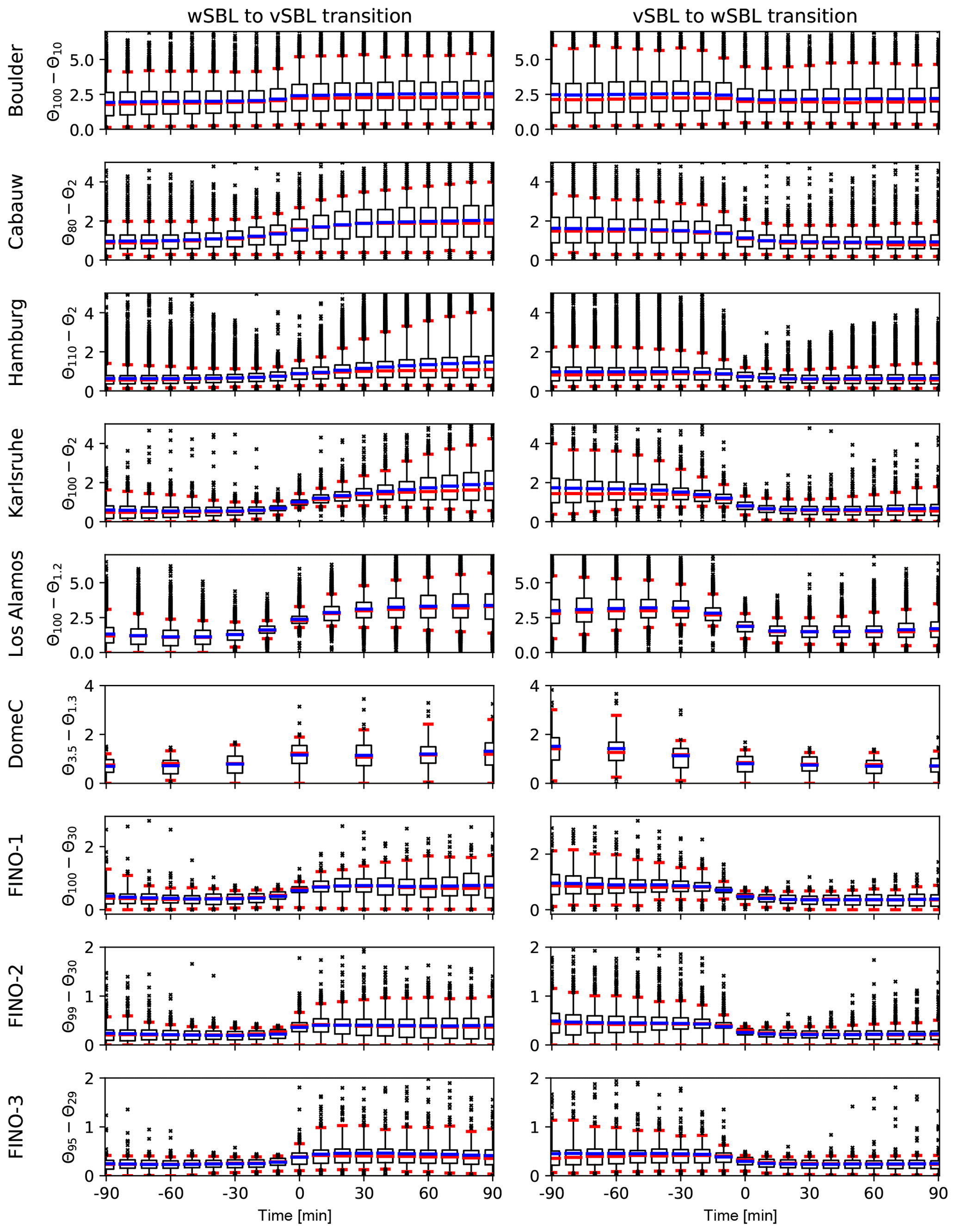
https://www.nonlin-processes-geophys.net/26/401/2019/npg-26-401-2019-f09

Figure 9Time evolution of the distribution of the stratification as estimated by the potential temperature difference between about 100 m and observations closest to the surface for land-based stations, between about 4 and 1 m for DomeC and between about 100 and 30 m for the sea-based stations in times of wSBL to vSBL (left) and vSBL to wSBL transitions (right). The distributions show the interquartile range (box), 5th to 95th percentile range (outer red bars), median, and mean values (or red and blue lines).

Download

The derived transition probabilities conditioned on Θ₁₀₀−Θ_s as estimated from VP_ref (binned by increments of 0.2 K) demonstrate qualitatively similar behaviour at all the stations (Fig. 8, second row). In contrast to conditioning on Ri_B, conditioning transition probabilities on stratification does not show marked differences between land- and sea-based stations. The $P (wSBL \to vSBL | Θ_{100} - Θ_{s})$ demonstrates an almost linear increase with increasing stability across all the tower sites. The turbulence recovery transition, on the other hand, shows very low $P (vSBL \to wSBL | Θ_{100} - Θ_{s})$ above about 2–3 K but increases rapidly for weaker inversion strengths. To build a state-dependent parameterization for S conditioned on stratification, conditional transition probabilities discussed above are fit to functional forms. As the wSBL cannot be sustained for strong inversions or a vSBL for weak inversions (Fig. 8, second row), transition probabilities for such conditions are set to 1. The functional forms for the stratification-dependent transition probabilities are

\begin{matrix} (4) & \begin{aligned} P & (wSBL \to vSBL | Θ_{100} - Θ_{s}) = \\ \{\begin{cases} α (Θ_{100} - Θ_{s}) + δ & for & Θ_{100} - Θ_{s} < 3 K \\ 1 & for & Θ_{100} - Θ_{s} \geq 3 K \end{cases} \end{aligned} \end{matrix}

and

\begin{matrix} (5) & \begin{aligned} P & (vSBL \to wSBL | Θ_{100} - Θ_{s}) = \\ α \tanh (\frac{Θ_{100} - Θ_{s} - β}{γ}) + δ . \end{aligned} \end{matrix}

The best-fit parameter and the RMSE for each station are listed in Table 4; the corresponding best-fit functions are shown in Fig. 8 (second row). Those fits are similar enough to each other to motivate analysis of the mean behaviour across all data, yielding parameter sets as listed in Table 4 and corresponding functions as depicted in Fig. 8 (third row, solid black line). Using the median parameter set or a best fit through all the data does not change the parameterization substantially.

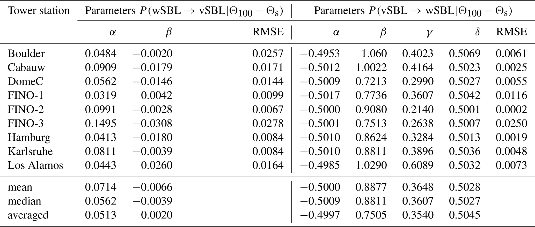
Table 4Parameter values for the state-dependent parametric probability transition functions conditioned on stratification (Θ₁₀₀−Θ_s, Θ₄−Θ_s, and Θ₁₀₀−Θ₃₀ for, respectively, land-, glacial-, and sea-based sites) and the RMSE between parameterized values and those obtained from estimations of HMM analyses. The mean and median values of the parameters are stated below together with the best-fit approximation through all data (averaged).

Download Print Version | Download XLSX

5.2 Stochastic forcing in the vSBL regime

As described in the Introduction, state-of-the-art planetary boundary layer turbulence parameterizations are able to produce radiatively driven turbulence collapse. In contrast, mechanisms to explicitly generate the turbulence recovery are too weak or lacking in standard parameterizations. He et al. (2012) showed that a stochastic process representing the effects of intermittent turbulence events can be implemented as an extra source term in the prognostic TKE budget during vSBL conditions, such that these events episodically drive the vSBL into a turbulence active regime. In their approach, however, the generation of intermittent turbulence bursts did not depend on the state of the boundary layer. Here, we propose to introduce a new local variable, the two-value discrete SBL regime occupation variable S, tracking SBL regimes. At each time step the occurrence of a regime transition is determined randomly using the instantaneous state-dependent transition probabilities derived above. When S is in the vSBL, additional stochastic forcing is added as a representation of the effect of intermittent turbulence bursts. These enhancements occur with random sizes and at random times and are similar to a compound Poisson process. This approach is designed to be able to reproduce the recovery time in the vSBL event duration distribution.

Many models, including the one we consider, represent turbulence fluxes using first-order closure. Here, we represent additional stochastic forcing in the vSBL by increasing the diffusivities of heat and momentum:

\begin{matrix} (6) & K (t, z) = K_{SCM} (t, z) + \sum_{k} {SF}_{k} (t, z), \end{matrix}

where K is the diffusivity for momentum and heat, K_SMC is the diffusivity as determined by the standard SCM parameterization (cf. Eq. B7), and SF_k represents the effects of the kth intermittent turbulence pulse parameterized as follows.

At each time step the probability of the occurrence of an intermittent turbulence pulse is given by λ_SF dt, where λ_SF is its occurrence rate and dt the model time step. If a turbulence pulse is determined to occur at time t_k, a random number r is drawn from a uniform distribution on [0,R] representing the maximum strength of the burst SF_k, occurring at time $t_{w_{k}} = t_{k} + τ_{w}$ .
The evolution of SF_k is split into growth and decay phases. The relatively short growth phase is introduced to avoid numerical instabilities, while the decay phase represents the dissipation of the intermittent turbulence pulse. Each SF_k is assumed to have a Gaussian profile in the vertical (which is intended to represent the localization of the enhanced mixing in the region where the turbulence pulse occurs) given by
$\begin{matrix} (7) & {SF}_{k} (t, z) = s_{k} (t) \exp (- \frac{(z - h_{k} (t))^{2}}{2 σ_{k}^{2} (t)}) . \end{matrix}$
The strength s_k(t) increases from t_k until $t_{w_{k}}$ according to a hyperbolic tangent function. Afterwards an exponential decay is prescribed with an eddy overturning timescale τ_e:
$\begin{matrix} (8) & \begin{aligned} s_{k} (t) = \\ \{\begin{aligned} 0 & for & t < t_{k} \\ 0.505 r \tanh (\frac{t - 0.5 τ_{w} - t_{w_{k}}}{0.5 τ_{w}} \\ \tanh^{- 1} (\frac{99}{101})) + 0.505 r & for & t_{k} \leq t < t_{w_{k}} \\ r \exp (- \frac{t - t_{w_{k}}}{τ_{e}}) & for & t \geq t_{w_{k}} \end{aligned} . \end{aligned} \end{matrix}$
We assume the centre of the turbulence pulse, h_k(t), to be initiated aloft (cf. AM19c, Fig. 4) and to move exponentially towards the surface during the decay phase:
$\begin{matrix} (9) & \begin{aligned} h_{k} (t) = \\ \{\begin{aligned} h_{b} & for & t < t_{w_{k}} \\ (h_{b} - h_{e}) \exp (- \frac{t - t_{w_{k}}}{τ_{h}}) + h_{e} & for & t \geq t_{w_{k}} \end{aligned}, \end{aligned} \end{matrix}$
where h_b and h_e denote the heights of the centre of SF_k(t,z) at the beginning and end of the turbulence pulse, respectively, and τ_h is the vertical migration timescale.
The width of SF_k(t,z), σ_k(t), is assumed to increase from the onset of the pulse until $t_{w_{k}}$ according to a hyperbolic tangent function which is introduced to avoid numerical instabilities as for s_k(t). The functional form ensures σ_k(t) increases in a similar way to s_k(t). During its decay σ_k(t) widens exponentially (representing the interaction of the turbulent patch with its surroundings) with a typical broadening timescale τ_σ:
$\begin{matrix} (10) & \begin{aligned} σ_{k} (t) = \\ \{\begin{aligned} \frac{σ_{w} + 1}{2} \tanh (\frac{t - 0.5 τ_{w} - t_{w_{k}}}{0.5 τ_{w}} \\ \tanh^{- 1} (\frac{σ_{w} - 1}{σ_{w} + 1})) + \frac{σ_{w} + 1}{2} & for & t < t_{w_{k}} \\ (σ_{w} - σ_{e}) \exp (- \frac{t - t_{w_{k}}}{τ_{σ}}) + σ_{e} & for & t \geq t_{w_{k}} \end{aligned}, \end{aligned} \end{matrix}$
where σ_w and σ_e are the widths of the turbulence pulse at, respectively, the time of its maximal strength and end of its lifecycle.

As indicated by Eq. (6), the effects of multiple overlapping turbulence bursts are taken to be additive. Thus, we assume no interaction between successive turbulence bursts. Below we test the parameterization in an idealized SCM. The values for the parameters in the stochastic forcing parameterization as used in the SCM experiments are listed in Table 5.

Table 5Values for the free parameters in the stochastic forcing parameterization as used in the SCM experiment.

Download Print Version | Download XLSX

5.3 SCM experiments with explicitly stochastic parameterization

The SCM we use to test the parameterization is described in van Hooijdonk et al. (2017) and Holdsworth and Monahan (2019). The governing equations of the SCM are presented in detail in Appendix B. In this study we consider the upper boundary of the model, at which we impose the boundary condition that the flow is geostrophic with a speed of 6 m s⁻¹, to be fixed at 5000 m. The lower boundary of the model domain is determined by the momentum roughness length which is set at z₀=0.001 m over a dry sand surface with density ρ_s=1600 kg m⁻³, specific heat capacity c_s=800 J kg⁻¹ K⁻¹, and thermal conductivity λ_s=0.3 W m⁻¹ K⁻¹. Furthermore, we assume clear-sky conditions.

The explicitly stochastic parameterization described above results in SBL transitions that are qualitatively in agreement with observations. An example realization is presented in Fig. 10. In this realization radiative cooling leads initially to a steady increase in stratification and flow stability. Once the vSBL is established (around simulation hour 2) turbulence pulses occur (none of which are individually sufficient to initiate a vSBL to wSBL transition). These turbulence pulses result in heat fluxes slightly larger than observed but of the right order of magnitude (e.g. Doran, 2004). The occurrence of multiple smaller turbulence pulses between simulation hours 6 and 7.5 slowly erodes the stratification until it is sufficiently weakened that a vSBL to wSBL transition occurs. Consistent with observations, the simulated vSBL to wSBL transition lags behind the occurrence of the last turbulence burst (AM19c). After the wSBL is established (about simulation hour 7.5) the stratification begins to increase again and a subsequent turbulence collapse occurs approximately 1.5 h later. This event duration is very close to the peak in the pdf of the wSBL event duration (cf. Fig. 4), providing further evidence that these recovery periods in the wSBL are related to internal dynamics.

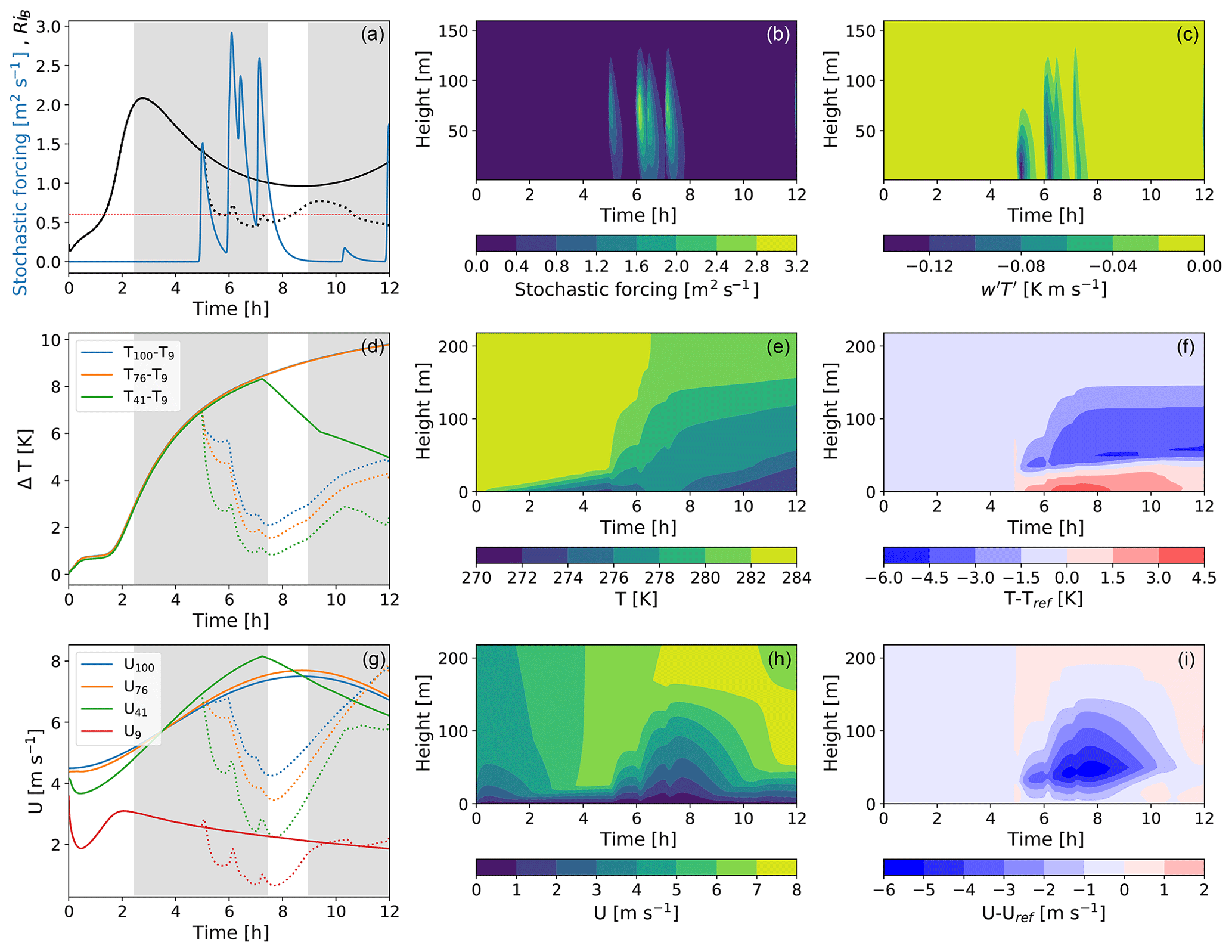
https://www.nonlin-processes-geophys.net/26/401/2019/npg-26-401-2019-f10

Figure 10One realization of a 12 h simulation of the evolution of the nocturnal boundary layer (with time zero being the time the net energy surface flux becomes negative) using the proposed parameterization. Times when S is in the vSBL are highlighted in grey. Top row from (a) to (c): Ri_B (solid and dotted black lines, respectively, for the reference experiment without the stochastic parameterization and the experiment with the stochastic parameterization) and the strength of the stochastic forcing (blue line; a); the structure of the stochastic forcing function (b) and the resulting kinematic heat fluxes (c). Middle row from (d) to (f): the stratification between different levels (d), the temperature profiles (e), and the difference in the temperature field to the reference experiment without the stochastic parameterization (f). Third row from (g) to (i): wind speeds at different heights (g), wind speed profiles (h), and the difference in the wind field to the reference experiment without the stochastic parameterization (i).

Download

Structures of wind and temperature profiles during vSBL to wSBL transitions resemble those of observations (cf. AM19c). Turbulence pulses lead to warming in the lowest 40 m of the boundary layer as turbulent sensible heat fluxes transport warm air from layers between 50 and 150 m towards the surface (Fig. 10d–f). Enhanced vertical momentum transport results in the near-surface winds first increasing and then decreasing (as a result of enhanced momentum flux into the surface; Fig. 10g–i). The relative magnitudes of the initial wind speed increase and subsequent decrease are sensitive to the height and width of SF_k (not shown). As the turbulence pulses decrease the stratification, boundary layer heights increase. These results demonstrate that an explicitly stochastic model with state-dependent transition probabilities and a representation of intermittent turbulence pulses in the vSBL can produce regime transitions that are in qualitative agreement with observations.

6 Discussion and conclusions

Recent studies have demonstrated that hidden Markov model (HMM) analysis is an effective tool to classify the nocturnal boundary layer (SBL) into weakly stable (wSBL) and very stable (vSBL) conditions (Monahan et al., 2015, AM19a, AM19b, AM19c). One goal of this study is to investigate whether a two-regime “freely running” stationary Markov chain (FSMC, obtained from the HMM analysis) is able to simulate SBL regime statistics with sufficient accuracy to be the foundation of a stochastic parameterization of SBL regimes. We have assessed the performance of the FSMC (using the most likely transition probabilities from HMM analyses) relative to the observed regime statistics such as the distributions of event durations and the probabilities of occurrence of very persistent nights (nights without SBL regime transitions), of any regime transitions, and of multiple subsequent transitions.

The non-stationary occurrence probabilities of very persistent nights as estimated from the HMM analyses cannot be accounted for in a FSMC. The occurrence of regime transitions is slightly overestimated by the FSMC. Transitions subsequent to preceding ones and the mean event durations in each regime are relatively close to the statistics as estimated with the HMM across all sites and seasons. The recovery time between regime transitions, however, is not explainable by any two-regime FSMC.

By fixing the persistence probability matrix and producing new perturbed HMM regime sequences we have quantified the range of persistence probabilities that are consistent with the most likely HMM regime sequence. At all the sites considered, we find that the HMM regime sequence varies only slightly for reasonable variations of transition probabilities.

Generally, no persistence probability range can be identified for which all SBL regime statistics of a FSMC are consistent with those of the HMM analysis. This result is true even when seasonal non-stationarity is accounted for. The non-Markov behaviour of regime occupation and the fact that aspects of regime transitions such as radiatively driven turbulence collapse can be simulated by models indicate the need for state-dependent transition probabilities in any explicitly stochastic representation of SBL regime transitions.

With the exception of the sea-based stations, state-dependent transition probabilities conditioned on the bulk Richardson number (Ri_B) exhibit a systematic state-dependent behaviour for wSBL to vSBL transitions. Transition probabilities for turbulence recovery events, on the other hand, demonstrate approximately state-independent characteristics with little consistency across sites. The lack of robustness of the conditional transition probabilities and weak dependence of turbulence recovery on Ri_B imply that Ri_B is not an appropriate conditioning variable.

State-dependent transition probabilities conditioned on stratification, in contrast, demonstrate a systematic state-dependent behaviour for both types of transitions across all stations. The wSBL to vSBL transition probabilities conditioned on the stratification increase almost linearly up to a threshold, while the vSBL to wSBL transition probabilities show a sigmoidal behaviour.

A prototype of an explicitly stochastic parameterization is developed based on the following foundations. The explicitly stochastic parameterization uses a new local variable S tracking the SBL regime (wSBL or vSBL). At each time step, the occurrence of a transition is determined randomly using the instantaneous state-dependent transition probabilities. If S is determined to be in the vSBL, episodes of enhanced turbulent mixing are added.

Experiments in an idealized SCM confirm that such an approach provides a reasonable representation of SBL regime dynamics. VSBL to wSBL transitions are related to the occurrence of turbulence bursts, lagging these slightly. The simulated responses of temperatures and wind speeds due to the enhanced heat and momentum fluxes towards the surface are comparable to observations. For both transitions, simulated recovery times are consistent with the observed distributions.

Emphasizing the fact that the explicitly stochastic parameterization presented here is only intended to be a proof of concept, preliminary results suggest that the parameterization has the potential to simulate SBL regime dynamics in weather and climate models. The observational information on climatological regime statistics and event duration distributions (cf. AM19b, AM19c, and the present study) can be used to tune the parameterization to generate the appropriate SBL regime variability. Due to the fact that event duration distributions and stratification-dependent transition probabilities are similar between the midlatitude tower sites, we believe that the transition process at those stations can be parameterized independently of the local complexity of the surface conditions (such as surface type or topography). Although at DomeC similar stratification-dependent transition probabilities can be obtained, the altitude range used to determine stratification is different than at the other sites, suggesting that a generalized parameterization has to take additional local state variables into account. Furthermore, even though a systematic behaviour of transition probabilities conditioned on Ri_B across the different tower sites is absent, Ri_B is a coarse approximation to Ri. Analyses of other data sets (with higher spatial and temporal resolution) allowing for better approximations or an estimation of the gradient Ri or Ri flux are needed to determine whether a systematic behaviour is truly absent.

As our model analysis only considers fixed surface and upper boundary conditions, sensitivity analyses of these conditions in the idealized SCM as well as of different resolutions in both time and space must be assessed in terms of different observational case studies. Due to the fact that the first-order closure requires us to consider the effects of intermittent turbulence events as an enhancement of diffusivities for momentum and heat, we have imposed a rather synthetic space–time structure of these enhancements. As intermittent turbulence events are associated with the local enhancement of turbulence kinetic energy (TKE), our parameterization of episodically occurring turbulence bursts can more naturally be implemented in a prognostic TKE scheme as an additional TKE source term (e.g. He et al., 2012, 2019). Such an approach would allow the model to determine the space–time structure of turbulence pulses as well as the interaction of turbulence bursts. In the future, we will implement the parameterization in a more complex SCM (with and without a prognostic TKE scheme) to obtain a more comprehensive assessment of its use in numerical weather prediction and climate models.

Finally, the parameterization requires further information regarding horizontal dependence of regime statistics, as it is not reasonable to expect an entire large-scale weather or climate model grid box to always be in one or the other state. This horizontal dependence will be the subject of a future study. Assessment of the dependence length scales relative to the grid box size will allow the determination of the effects of spatial averaging to the grid box scale on the probability distribution of SBL quantities.

Data availability

The observational data can be obtained from the persons and sources indicated in the acknowledgments. Data from the single-column model can be obtained from https://doi.org/10.5683/SP2/ZUENCK (Abraham et al., 2019).

Appendix A

In this Appendix, we present the calculations of quantities based on “freely running” stationary Markov chains. Note that we introduce in the following equations the notation of $P (i_{t - 1} \to i_{t})$ instead of $Q_{i_{t} i_{t - 1}}$ (cf. Eq. 2) indicating the regime transition probabilities between two time steps. We replace the mathematical notation of $i \in {0, 1}$ for the regime occupation with the terms wSBL and vSBL in order to increase the readability.

A1 Calculation of very persistent regimes

The occurrence probability of very persistent SBL nights in a stationary Markov chain is calculated using the persistence probabilities of the Markov chain (i.e. P(wSBL→wSBL) and P(vSBL→vSBL)) as follows:

\begin{array}{l} (A1) & P r (wSBL | n) & = π_{wSBL} P (wSBL \to wSBL)^{n}, \\ (A2) & P r (vSBL | n) & = π_{vSBL} P (vSBL \to vSBL)^{n}, \end{array}

where π_wSBL and π_vSBL are, respectively, the initial climatological distributions of being in the wSBL or vSBL and n equals the length of the night in hours multiplied by 6 (for a data resolution of 10 min).

A2 Calculation of at least one particular SBL transition occurrence

The probability of the occurrence of a particular SBL transition in a night of duration n can be expressed in terms of the probability of the absence of any transitions and the probability of a single complementary transition. In the case of the wSBL to vSBL transition, the single complementary transitions are from the vSBL to the wSBL. Naturally, the reverse is true for vSBL to wSBL transitions. That way we account for all possibilities that definitely do not have a transition of the desired type.

The probability of the occurrence of turbulence collapse is

\begin{matrix} (A3) & \begin{aligned} P r ((wSBL \to vSBL | n) > 0) = 1 \\ - \underset{prob. of remaining in the wSBL}{\underset{︸}{π_{wSBL} P (wSBL \to wSBL)^{n}}} - \underset{prob. of remaining in the vSBL}{\underset{︸}{π_{vSBL} P (vSBL \to vSBL)^{n}}} \\ - \underset{prob. of only vSBL to wSBL transitions, remaining in the wSBL afterwards}{\underset{︸}{\sum_{t = 0}^{n - 1} π_{vSBL} P (vSBL \to vSBL)^{t} P (vSBL \to wSBL) P (wSBL \to wSBL)^{n - t - 1}}} . \end{aligned} \end{matrix}

Equivalently, the probability of a turbulence recovery (vSBL to wSBL transition) is given by

\begin{matrix} (A4) & \begin{aligned} P r ((vSBL \to wSBL | n) > 0) = 1 \\ - \underset{prob. of remaining in the wSBL}{\underset{︸}{π_{wSBL} P (wSBL \to wSBL)^{n}}} - \underset{prob. of remaining in the vSBL}{\underset{︸}{π_{vSBL} P (vSBL \to vSBL)^{n}}} \\ - \underset{prob. of only wSBL to vSBL transitions, remaining in the vSBL afterwards}{\underset{︸}{\sum_{t = 0}^{n - 1} π_{wSBL} P (wSBL \to wSBL)^{t} P (wSBL \to vSBL) P (vSBL \to vSBL)^{n - t - 1}}} . \end{aligned} \end{matrix}

A3 Calculation of the probability of subsequent turbulence recovery or collapse event occurrences

The probability that a turbulence recovery event will occur after a turbulence collapse in a night of duration n time steps is equal to the sum of the probabilities of all events that include the occurrence of SBL patterns starting at time t₁ in the wSBL, and afterwards showing the sequence $wSBL \to \overset{t \times}{\overset{︷}{vSBL \to \dots \to vSBL}} \to wSBL$ with no further subsequent recovery events; i.e. the SBL remains in the wSBL or has a maximum of one more collapse. The last part of this calculation assures that no double counting of sequences with length t occurs as the probability calculation of being in the wSBL at time t₁ does not include information of the preceding path. The probability of a certain subsequent recovery pattern of length t can then be calculated as

\begin{matrix} (A5) & \begin{aligned} P r ((wSBL \to \overset{t \times}{\overset{︷}{vSBL \to \dots \to vSBL}} \to wSBL | n) > 0) \\ = \sum_{t_{1} = 0}^{n - t - 2} {(π^{T} Q^{t_{1}})}_{wSBL} P (wSBL \to vSBL) P {(vSBL \to vSBL)}^{t} \\ P (vSBL \to wSBL) [P {(wSBL \to wSBL)}^{n - t - t_{1} - 2} \\ + \sum_{t_{2} = 0}^{n - t - t_{1} - 3} P {(wSBL \to wSBL)}^{t_{2}} P (wSBL \to vSBL) \\ P {(vSBL \to vSBL)}^{n - t - t_{1} - t_{2} - 3}], \end{aligned} \end{matrix}

where π is the vector of climatological initial probabilities. Calculating the overall probability that such a subsequent event will occur is then the summation over all possible t:

\begin{matrix} (A6) & \begin{aligned} \sum_{t} P r ((wSBL \to \overset{t \times}{\overset{︷}{vSBL \to \dots \to vSBL}} \to wSBL | n) > 0) \\ = \sum_{t = 0}^{n - 2} \sum_{t_{1} = 0}^{n - t - 2} {(π^{T} Q^{t_{1}})}_{wSBL} P (wSBL \to vSBL) P {(vSBL \to vSBL)}^{t} \\ P (vSBL \to wSBL) [P {(wSBL \to wSBL)}^{n - t - t_{1} - 2} \\ + \sum_{t_{2} = 0}^{n - t - t_{1} - 3} P {(wSBL \to wSBL)}^{t_{2}} P (wSBL \to vSBL) \\ P {(vSBL \to vSBL)}^{n - t - t_{1} - t_{2} - 3}] . \end{aligned} \end{matrix}

Equivalently, the probabilities of subsequent turbulence collapses after recovery events are

\begin{matrix} (A7) & \begin{aligned} P r ((vSBL \to \overset{t \times}{\overset{︷}{wSBL \to \dots \to wSBL}} \to vSBL | n) > 0) \\ = \sum_{t_{1} = 0}^{n - t - 2} {(π^{T} Q^{t_{1}})}_{vSBL} P (vSBL \to wSBL) P {(wSBL \to wSBL)}^{t} \\ P (wSBL \to vSBL) [P {(vSBL \to vSBL)}^{n - t - t_{1} - 2} \\ + \sum_{t_{2} = 0}^{n - t - t_{1} - 3} P {(vSBL \to vSBL)}^{t_{2}} P (vSBL \to wSBL) \\ P {(wSBL \to wSBL)}^{n - t - t_{1} - t_{2} - 3}] . \end{aligned} \end{matrix}

Calculating the overall probability that such a subsequent event will occur is then the summation over all possible t:

\begin{matrix} (A8) & \begin{aligned} \sum_{t} P r ((vSBL \to \overset{t \times}{\overset{︷}{wSBL \to \dots \to wSBL}} \to vSBL | n) > 0) \\ = \sum_{t = 0}^{n - 2} \sum_{t_{1} = 0}^{n - t - 2} {(π^{T} Q^{t_{1}})}_{vSBL} P (vSBL \to wSBL) P {(wSBL \to wSBL)}^{t} \\ P (wSBL \to vSBL) [P {(vSBL \to vSBL)}^{n - t - t_{1} - 2} \\ + \sum_{t_{2} = 0}^{n - t - t_{1} - 3} P {(vSBL \to vSBL)}^{t_{2}} P (vSBL \to wSBL) \\ P {(wSBL \to wSBL)}^{n - t - t_{1} - t_{2} - 3}] . \end{aligned} \end{matrix}

Appendix B

The idealized SCM is a model of pressure-driven flow in the dry SBL assuming horizontal homogeneity, described in detail in Holdsworth and Monahan (2019). The model equations follow those of Blackadar (1979):

\begin{array}{l} (B1) & \frac{\partial U}{\partial t} & = \frac{1}{ρ} \frac{\partial τ_{x}}{\partial z} - \frac{1}{ρ} \frac{\partial p}{\partial x} + f_{0} V, \\ (B2) & \frac{\partial V}{\partial t} & = \frac{1}{ρ} \frac{\partial τ_{y}}{\partial z} - \frac{1}{ρ} \frac{\partial p}{\partial y} - f_{0} U, \\ (B3) & \frac{\partial T}{\partial t} & = - \frac{1}{ρ c_{p}} \frac{\partial H}{\partial z} - C_{HL}, \\ (B4) & \frac{\partial T_{s}}{\partial t} & = C_{1} (I_{l w} - σ T_{s}^{4} - H_{0}) - C_{2} (T_{s} - T_{d}), \end{array}

where the three state variables U(z,t), V(z,t), and T(z,t) are the zonal velocity, meridional velocity, and potential temperature. The surface temperature T_s is determined by the sum of radiative fluxes, turbulent sensible heat fluxes, and surface heat fluxes as described in more detail below. The constant C_HL=2 K h⁻¹ represents the atmospheric cooling due to net longwave radiative flux divergence and is set as a fixed constant for simplicity.

The geostrophic wind components are defined by

\begin{array}{l} (B5) & U_{g} & = - \frac{1}{f_{0} ρ} \frac{\partial p}{\partial y}, \\ (B6) & V_{g} & = \frac{1}{f_{0} ρ} \frac{\partial p}{\partial x}, \end{array}

with the magnitude of the geostrophic wind speed given by $S_{g} = (U_{g}^{2} + V_{g}^{2})^{0.5}$ .

The vertical heat flux $H = ρ c_{p} \overline{w^{'} T^{'}}$ and shear stresses $τ_{x} = - ρ \overline{U^{'} w^{'}}$ and $τ_{y} = - ρ \overline{V^{'} w^{'}}$ (where w is the vertical velocity) are parameterized using first-order closure $τ_{x} / ρ = K_{m} \partial_{z} U$ , $τ_{y} / ρ = K_{m} \partial_{z} V$ , and $H / ρ c_{p} = - K_{H} \partial_{z} T$ , where K_m and K_h are the diffusivities for, respectively, momentum and heat. The diffusivities are taken to be the sum of molecular and turbulent contributions (Moene et al., 2010):

\begin{array}{l} (B7) & K_{m} & = l^{2} | \partial_{z} U | f_{m} (R i) + ν, \\ (B8) & K_{h} & = l^{2} | \partial_{z} U | f_{h} (R i) + λ, \end{array}

where the molecular contribution $ν = 1.5 \times 10^{- 5} m^{2} s^{- 1}$ is the kinematic viscosity. The molecular Prandtl number is fixed at Pr=0.72 and $λ = ν / P r$ is the molecular diffusivity. The mixing length is given by

\begin{matrix} (B9) & l = (1 - \exp (- \frac{u_{0 *} z}{C ν})) (\frac{κ (z - z_{0})}{(1 + κ (z - z_{0}) / λ_{0})}), \end{matrix}

with κ the von Kármán constant, u_* friction velocity, C=26 (Van Driest, 1951), and $λ_{0} = 0.00027 S_{g} / f_{0}$ (Blackadar, 1962).

The stability functions f_m,h(Ri) depend on the Richardson number $R i = \frac{g}{T_{REF}} \frac{\partial_{z} T}{(\partial_{z} U)^{2}}$ and are related to the similarity functions from MOST ϕ_m,h(ζ) by

\begin{matrix} (B10) & \begin{aligned} f_{m} (R i_{eq}) & = ϕ_{m}^{- 2} (ζ), \\ f_{h} (R i_{eq}) & = ϕ_{m}^{- 1} (ζ) ϕ_{h}^{- 1} (ζ), \end{aligned} \end{matrix}

where $ζ = z / L$ is the stability parameter and $L = - \frac{u_{*}^{2}}{κ \frac{g}{T_{s}} \frac{H_{0}}{c_{p} ρ}}$ is the Obukhov length. In our simulations, we use the Businger–Dyer formulation given by $ϕ_{m, h} (ζ) = 1 + β ζ$ , where $β = 1 / R i_{c} = 5.2$ (Businger, 1988).

At the upper boundary of the model we impose the boundary condition that the flow is geostrophic and a no-flux condition so H=0 and τ=0. The lower boundary of the model domain is determined by the roughness length (assumed to be the same for momentum and energy) with no-slip boundary conditions U(z₀)=0 and $T (z_{0}, t) = T_{s} (t)$ .

The model implements the surface energy scheme of Blackadar (1976), known as the force-restore method. The surface, represented as an infinitesimally thin layer with temperature T_s(t) at z=z₀, is forced by the net radiation and sensible heat flux and restored to the subsurface temperature through the subsurface energy fluxes. The damping depth of the diurnal forcing $d = (2 λ_{s} / C_{s} ω)^{0.5}$ , where C_s=ρ_sc_s is the volumetric heat capacity, is associated with a sinusoidal diurnal forcing. The temperature at this depth is set as the subsurface temperature T_d=281 K. In Eq. (B4), $C_{1} = 2 / (0.95 C_{s} d)$ and $C_{2} = 1.18 (2 π / T_{d})$ . The first two terms in Eq. (B4) constitute the net longwave radiation Q_n, the third term is the sensible heat flux into the atmosphere due to turbulent transports H₀, and the fourth term is the heat flux into the subsurface G. As our focus is on the stably stratified boundary layer we do not include the effects of albedo or latent heat in the heat budget. We also neglect the effects of the vegetation canopy.

The downwelling longwave radiation is given by

\begin{matrix} (B11) & I_{lw} = σ (Q_{c} + 0.67 (1 - Q_{c}) {(1670 Q_{a})}^{0.08}) T_{a}^{4}, \end{matrix}

where Q_c is the cloud fraction, Q_a is the specific humidity, and T_a is the atmospheric temperature at a reference level z_a just above the Earth's surface (Staley and Jurica, 1972; Deardorff, 1978). For simplicity, Q_a is held constant at 0.003 kg kg⁻¹.

The equations are integrated in time using a fourth-order Runge–Kutte method. The spatial discretization is obtained using finite differences on a logarithmic grid. This grid has 50 vertical levels with a much finer resolution in the boundary layer than aloft and is determined by $z_{j} = Δ z_{0} \frac{r^{j} - 1}{r - 1}$ with a stretch factor $r = \frac{Δ z_{j}}{Δ z_{j - 1}} ≃ 1.10$ and an initial step size of Δz₀=2 m. The prognostic variables U,V, and T are defined at the z_i grid levels, while the diagnostic variables of H, τ, and Ri are defined at the z_i+½ levels.

We define t=0 as the time when the shortwave radiation goes to zero, acknowledging the fact that observations indicate that the onset of the SBL can occur before this time (van Hooijdonk et al., 2017; van de Wiel et al., 2017, AM19a). The initial conditions were set in accordance with the logarithmic equations that arise from MOST. The near-neutral profiles for temperature and wind used to initialize the model are given by

\begin{matrix} (B12) & \begin{aligned} U_{0} & = \frac{U_{ext}}{κ} \ln (z / z_{0}), \\ V_{0} & = \frac{V_{ext}}{κ} \ln (z / z_{0}), \\ T_{0} & = T_{s} + \frac{θ_{ext}}{κ} \ln (z / z_{0}) . \end{aligned} \end{matrix}

where $U_{ext} = U_{g} κ / \ln (h / z_{0})$ , $V_{ext} = V_{g} κ / \ln (h / z_{0})$ , and θ_ext=0.01 K (Monin and Obukhov, 1954). For simplicity, we set $\frac{\partial p}{\partial y} = 0$ in all of our simulations, so U₀ is identically zero at the start of the simulation.

Author contributions

The authors developed the ideas underlying this study together. CA executed the analysis and designed the draft of this manuscript. All authors contributed to improving the manuscript.

Competing interests

The authors declare that they have no conflict of interest.

Acknowledgements

We would like to thank a number of individuals and institutes for their willingness to share their tower data which were indispensable in carrying out this extensive comparison of SBL structures at different location sites. Our acknowledgements are presented in the order that the tower stations were presented in the paper, but we are equally thankful to all. The NOAA Earth System Research Laboratory's (ESRL) Physical Sciences Division (PSD) operates the Boulder Atmospheric Observatory (BAO) tower and makes the data publicly available. Information how to obtain the data is given at https://www.esrl.noaa.gov/psd/technology/bao/site/ (last access: 12 November 2019). The Royal Dutch Meteorological Institute (KNMI) is thanked for providing tower data from the Cabauw Experimental Site for Atmospheric Research (CESAR) which can be downloaded at http://www.cesar-database.nl (last access: 12 November 2019). Felix Ament and Ingo Lange provided data from the Wettermast Hamburg of the Meteorological Institute of the University of Hamburg. Martin Kohler and the Institute for Meteorology and Climate Research of the Karlsruhe Institute of Technology (KIT) provided observations from the turbulence and meteorological mast in Karlsruhe. The team of the Los Alamos National Laboratory (LANL) are thanked for making data from the Environmental Monitoring Plan (EMP) freely available which can be downloaded from https://envweb.lanl.gov/weathermachine/data_request_green_weather.asp (last access: 12 November 2019). The French and Italian polar institutes (IPEV and PANRA, respectively) which operate the DomeC observatory in Antarctica are acknowledged for providing data through IPEV (program CALVA 1013), INSU/LEFE (GABLS4 and DEPHY2), and OSUG (GLACIOCLIM). The data were obtained on 22 May 2017 from http://www.lmd.jussieu.fr/~cgenthon/SiteCALVA/. Further information can be obtained from Christophe Genthon. The Bundesamt für Seeschifffahrt und Hydrographie (BSH), the Bundesministeriums für Wirtschaft und Energie (BMWi), the Projektträger Jülich (PTJ), and Olaf Outzen are thanked for granting access to the data from the offshore research platforms FINO-1, FINO-2, and FINO-3 in Germany.

Carsten Abraham and Adam H. Monahan are supported by the Natural Sciences and Engineering Research Council Canada (NSERC). Amber M. Holdsworth acknowledges support by the DFO ACCASP program.

Finally, we thank three anonymous reviewers whose suggestions substantially improved this paper.

Financial support

This research has been supported by the Natural Sciences and Engineering Research Council Canada (NSERC grant).

Review statement

This paper was edited by Juan Restrepo and reviewed by three anonymous referees.

References

Abraham, C. and Monahan, A. H.: Climatological Features of the Weakly and Very Stably Stratified Nocturnal Boundary Layers, Part I: State Variables Containing Information about Regime Occupation, J. Atmos. Sci., 76, 3455–3484, https://doi.org/10.1175/JAS-D-18-0261.1, 2019a. a

Abraham, C. and Monahan, A. H.: Climatological Features of the Weakly and Very Stably Stratified Nocturnal Boundary Layers. Part II: Regime Occupation and Transition Statistics and the Influence of External Drivers, J. Atmos. Sci., 76, 3485–3504, https://doi.org/10.1175/JAS-D-19-0078.1, 2019b. a

Abraham, C. and Monahan, A. H.: Climatological Features of the Weakly and Very Stably Stratified Nocturnal Boundary Layers, Part III: The Structure of Meteorological State Variables in Persistent Regime Nights and across Regime Transitions, J. Atmos. Sci., 76, 3505–3527, https://doi.org/10.1175/JAS-D-18-0274.1, 2019c. a

Abraham, C., Holdsworth, A. M., and Monahan, A. H.: Replication Data for: A prototype stochastic parameterization of regime behaviour in the stably stratified atmospheric boundary layer, https://doi.org/10.5683/SP2/ZUENCK, Scholars Portal Dataverse, 2019.

Acevedo, O. C. and Fitzjarrald, D. R.: In the Core of the Night-Effects of Intermittent Mixing on a Horizontally Heterogeneous Surface, Bound-Lay. Meteorol., 106, 1–33, https://doi.org/10.1023/A:1020824109575, 2003. a

Acevedo, O. C., Moraes, O. L. L., Degrazia, G. A., and Medeiros, L. E.: Intermittency and the Exchange of Scalars in the Nocturnal Surface Layer, Bound.-Lay. Meteorol., 119, 41–55, https://doi.org/10.1007/s10546-005-9019-3, 2006. a

Acevedo, O. C., Mahrt, L., Puhales, F. S., Costa, F. D., Medeiros, L. E., and Degrazia, G. A.: Contrasting structures between the decoupled and coupled states of the stable boundary layer, Q. J. Roy. Meteorol. Soc., 142, 693–702, https://doi.org/10.1002/qj.2693, 2016. a

Acevedo, O. C., Maroneze, R., Costa, F. D., Puhales, F. S., Nogueira Martins, L. G., Soares de Oliveira, P. E., and Mortarini, L.: The Nocturnal Boundary Layer Transition from Weakly to Very Stable, Part 1: Observations, Q. J. Roy. Meteorol. Soc., https://doi.org/10.1002/qj.3642, 2019. a

Ansorge, C. and Mellado, J. P.: Global Intermittency and Collapsing Turbulence in the Stratified Planetary Boundary Layer, Bound.-Lay. Meteorol., 153, 89–116, https://doi.org/10.1007/s10546-014-9941-3, 2014. a, b

Baas, P., Bosveld, F. C., Baltink, H. K., and Holtslag, A. A. M.: A Climatology of Nocturnal Low-Level Jets at Cabauw, J. Appl. Meteorol. Climatol., 48, 1627–1642, https://doi.org/10.1175/2009JAMC1965.1, 2009. a

Banta, R. M., Mahrt, L., Vickers, D., Sun, J., Balsley, B. B., Pichugina, Y. L., and Williams, E. J.: The Very Stable Boundary Layer on Nights with Weak Low-Level Jets, J. Atmos. Sci., 64, 3068–3090, https://doi.org/10.1175/JAS4002.1, 2007. a, b

Barthlott, C., Kalthoff, N., and Fiedler, F.: Influence of high-frequency radiation on turbulence measurements on a 200 m tower, Meteorol. Z, 12, 67–71, https://doi.org/10.1127/0941-2948/2003/0012-0067, 2003. a

Basu, S., Porté-agel, F., Foufoula-Georgiou, E., Vinuesa, J.-F., and Pahlow, M.: Revisiting the Local Scaling Hypothesis in Stably Stratified Atmospheric Boundary-Layer Turbulence: an Integration of Field and Laboratory Measurements with Large-Eddy Simulations, Bound.-Lay. Meteorol., 119, 473–500, https://doi.org/10.1007/s10546-005-9036-2, 2006. a

Bechtold, P., Köhler, M., Jung, T., Doblas-Reyes, F., Leutbecher, M., Rodwell, M. J., Vitart, F., and Balsamo, G.: Advances in simulating atmospheric variability with the ECMWF model: From synoptic to decadal time-scales, Q. J. Roy. Meteorol. Soc., 134, 1337–1351, https://doi.org/10.1002/qj.289, 2008. a

Beeken, A., Neumann, T., and Westerhellweg, A.: Five Years of Operation of the First Offshore Wind Research Platform in the German Bight – FINO1, Tech. rep., German Wind Energy Institute (DEWI GmbH), DEWEK, DEWI GmbH, Ebertstraße 96, 26382 Wilhelmshaven, available at: http://www.dewi.de/dewi/fileadmin/pdf/publications/Publikations/5_Beeken.pdf (last access: 12 November 2019), 2008. a

Blackadar, A.: Modeling the nocturnal boundary layer, in: Proceedings of the Third Symposium on Atmospheric Turbulence, Diffusion and Air Quality, 46–49, American Meteorological Society, Boston, Mass., 1976. a

Blackadar, A.: High resolution models of the planetary boundary layer, Adv. Environ. Sci. Eng., 1, 50–85, 1979. a

Blackadar, A. K.: The vertical distribution of wind and turbulent exchange in a neutral atmosphere, J. Geophys. Res., 67, 3095–3102, https://doi.org/10.1029/JZ067i008p03095, 1962. a

Blumen, W.: An observational study of instability and turbulence in nighttime drainage winds, Bound.-Lay. Meteorol., 28, 245–269, https://doi.org/10.1007/BF00121307, 1984. a

Blumen, W., Banta, R., Burns, S. P., Fritts, D. C., Newsom, R., Poulos, G. S., and Sun, J.: Turbulence statistics of a Kelvin–Helmholtz billow event observed in the night-time boundary layer during the Cooperative Atmosphere–Surface Exchange Study field program, Dyn. Atmos. Oceans, 34, 189–204, https://doi.org/10.1016/S0377-0265(01)00067-7, 2001. a

Bosveld, F. C., Baas, P., Steeneveld, G.-J., Holtslag, A. A. M., Angevine, W. M., Bazile, E., de Bruijn, E. I. F., Deacu, D., Edwards, J. M., Ek, M., Larson, V. E., Pleim, J. E., Raschendorfer, M., and Svensson, G.: The Third GABLS Intercomparison Case for Evaluation Studies of Boundary-Layer Models. Part B: Results and Process Understanding, Bound.-Lay. Meteorol., 152, 157–187, https://doi.org/10.1007/s10546-014-9919-1, 2014. a, b

Bowen, B. M., Baars, J. A., and Stone, G. L.: Nocturnal Wind Direction Shear and Its Potential Impact on Pollutant Transport, J. Appl. Meteorol. Climatol., 39, 437–445, https://doi.org/10.1175/1520-0450(2000)039<0437:NWDSAI>2.0.CO;2, 2000. a

Brümmer, B., Lange, I., and Konow, H.: Atmospheric boundary layer measurements at the 280 m high Hamburg weather mast 1995–2011: mean annual and diurnal cycles, Meteorol. Z., 21, 319–335, https://doi.org/10.1127/0941-2948/2012/0338, 2012. a

Businger, J.: A note on the Businger-Dyer profiles, Bound.-Lay. Meteorol., 42, 145–151, https://doi.org/10.1007/BF00119880, 1988. a

Coulter, R. L. and Doran, J. C.: Spatial and Temporal Occurrences of Intermittent Turbulence During CASES-99, Bound.-Lay. Meteorol., 105, 329–349, https://doi.org/10.1023/A:1019993703820, 2002. a

Deardorff, J. W.: Efficient prediction of ground surface temperature and moisture, with inclusion of a layer of vegetation, J. Geophys. Res.-Oceans, 83, 1889–1903, https://doi.org/10.1029/JC083iC04p01889, 1978. a

Dempster, A. P., Laird, N. M., and Rubin, D. B.: Maximum Likelihood from Incomplete Data via the EM Algorithm, J. Roy. Stat. Soc., 39B, 1–38, 1979. a

Derbyshire, S. H.: Boundary-Layer Decoupling over Cold Surfaces as a Physical Boundary-Instability, Bound.-Lay. Meteorol., 90, 297–325, https://doi.org/10.1023/A:1001710014316, 1999. a

Dethloff, K., Abegg, C., Rinke, A., Hebestadt, I., and Romanov, V. F.: Sensitivity of Arctic climate simulations to different boundary-layer parameterizations in a regional climate model, Tellus A, 53, 1–26, https://doi.org/10.1034/j.1600-0870.2001.01073.x, 2001. a

Donda, J. M. M., van Hooijdonk, I. G. S., Moene, A. F., Jonker, H. J. J., van Heijst, G. J. F., Clercx, H. J. H., and van de Wiel, B. J. H.: Collapse of turbulence in stably stratified channel flow: a transient phenomenon, Q. J. Roy. Meteorol. Soc., 141, 2137–2147, https://doi.org/10.1002/qj.2511, 2015. a

Doran, J. C.: Characteristics of Intermittent Turbulent Temperature Fluxes in Stable Conditions, Bound.-Lay. Meteorol., 112, 241–255, https://doi.org/10.1023/B:BOUN.0000027907.06649.d0, 2004. a, b

Dörenkämper, M., Witha, B., Steinfeld, G., Heinemann, D., and Kühn, M.: The impact of stable atmospheric boundary layers on wind-turbine wakes within offshore wind farms, J. Wind Eng. Ind. Aerodynam., 144, 146–153, https://doi.org/10.1016/j.jweia.2014.12.011, 2015. a, b

Edwards, J. M., McGregor, J. R., Bush, M. R., and Bornemann, F. J. A.: Assessment of numerical weather forecasts against observations from Cardington: seasonal diurnal cycles of screen-level and surface temperatures and surface fluxes, Q. J. Roy. Meteorol. Soc., 137, 656–672, https://doi.org/10.1002/qj.742, 2011. a

Fischer, J.-G., Senet, C., Outzen, O., Schneehorst, A., and Herklotz, K.: Regional oceanographic distincions in the South-Eastern part of the North Sea: Results of two years of monitoring at the research platforms FINO1 and FINO3, in: German Wind Energy Conference DEWEK 2012, edited by: J.-G. Fischer, Bremen, Germany, 2012. a, b

Floors, R., Peña, A., and Gryning, S.-E.: The effect of baroclinicity on the wind in the planetary boundary layer, Q. J. Roy. Meteorol. Soc., 141, 619–630, https://doi.org/10.1002/qj.2386, 2014. a

Flores, O. and Riley, J. J.: Analysis of Turbulence Collapse in the Stably Stratified Surface Layer Using Direct Numerical Simulation, Bound.-Lay. Meteorol., 139, 241–259, https://doi.org/10.1007/s10546-011-9588-2, 2011. a

Franzke, C., Horenko, I., Majda, A. J., and Klein, R.: Systematic Metastable Atmospheric Regime Identification in an AGCM, J. Atmos. Sci., 66, 1997–2012, https://doi.org/10.1175/2009JAS2939.1, 2009. a

Fu, G., Charles, S. P., and Kirshner, S.: Daily rainfall projections from general circulation models with a downscaling nonhomogeneous hidden Markov model (NHMM) for south-eastern Australia, Hydrol. Process., 27, 3663–3673, https://doi.org/10.1002/hyp.9483, 2013. a

Genthon, C., Town, M. S., Six, D., Favier, V., Argentini, S., and Pellegrini, A.: Meteorological atmospheric boundary layer measurements and ECMWF analyses during summer at Dome C, Antarctica, J. Geophys. Res.-Atmos., 115, D5, https://doi.org/10.1029/2009JD012741, 2010. a

Genthon, C., Six, D., Gallée, H., Grigioni, P., and Pellegrini, A.: Two years of atmospheric boundary layer observations on a 45 m tower at Dome C on the Antarctic plateau, J. Geophys. Res.-Atmos., 118, 3218–3232, https://doi.org/10.1002/jgrd.50128, 2013. a

Gerbig, C., Körner, S., and Lin, J. C.: Vertical mixing in atmospheric tracer transport models: error characterization and propagation, Atmos. Chem. Phys., 8, 591–602, https://doi.org/10.5194/acp-8-591-2008, 2008. a

Grachev, A. A., Fairall, C. W., Persson, P. O. G., Andreas, E. L., and Guest, P. S.: Stable Boundary-Layer Scaling Regimes: The SHEBA Data, Bound.-Lay. Meteorol., 116, 201–235, https://doi.org/10.1007/s10546-004-2729-0, 2005. a

Grachev, A. A., Andreas, E. L., Fairall, C. W., Guest, P. S., and Persson, P. O. G.: The Critical Richardson Number and Limits of Applicability of Local Similarity Theory in the Stable Boundary Layer, Bound.-Lay. Meteorol., 147, 51–82, https://doi.org/10.1007/s10546-012-9771-0, 2013. a

Gryning, S.-E., Floors, R., Peña, A., Batchvarova, E., and Brümmer, B.: Weibull Wind-Speed Distribution Parameters Derived from a Combination of Wind-Lidar and Tall-Mast Measurements Over Land, Coastal and Marine Sites, Bound.-Lay. Meteorol., 159, 329–348, https://doi.org/10.1007/s10546-015-0113-x, 2016. a

He, Y., Monahan, A. H., Jones, C. G., Dai, A., Biner, S., Caya, D., and Winger, K.: Probability distributions of land surface wind speeds over North America, J. Geophys. Res.-Atmos., 115, D04103, https://doi.org/10.1029/2008JD010708, 2010. a

He, Y., McFarlane, N. A., and Monahan, A. H.: The Influence of Boundary Layer Processes on the Diurnal Variation of the Climatological Near-Surface Wind Speed Probability Distribution over Land, J. Climate, 115, D04103, https://doi.org/10.1175/JCLI-D-11-00321.1, 2012. a, b, c, d, e

He, Y., McFarlane, N. A., and Monahan, A. H.: A New TKE-Based Parameterization of Atmospheric Turbulence in the Canadian Global and Regional Climate Models, J. Adv. Model. Earth Sy., 11, 1153–1188, https://doi.org/10.1029/2018MS001532, 2019. a

Holdsworth, A. M. and Monahan, A. H.: Turbulent collapse and recovery in the stable boundary layer using an idealized model of pressure-driven flow with a surface energy budget, J. Atmos. Sci., 76, 1307–1327, https://doi.org/10.1175/JAS-D-18-0312.1, 2019. a, b, c, d, e

Holdsworth, A. M., Rees, T., and Monahan, A. H.: Parameterization Sensitivity and Instability Characteristics of the Maximum Sustainable Heat Flux Framework for Predicting Turbulent Collapse, J. Atmos. Sci., 73, 3527–3540, https://doi.org/10.1175/JAS-D-16-0057.1, 2016. a

Holtslag, A. A. M., Svensson, G., Baas, P., Basu, S., Beare, B., Beljaars, A. C. M., Bosveld, F. C., Cuxart, J., Lindvall, J., Steeneveld, G. J., Tjernström, M., and Wiel, B. J. H. V. D.: Stable Atmospheric Boundary Layers and Diurnal Cycles: Challenges for Weather and Climate Models, B. Am. Meteor. Soc., 94, 1691–1706, https://doi.org/10.1175/BAMS-D-11-00187.1, 2013. a, b, c, d

Horenko, I.: On the Identification of Nonstationary Factor Models and Their Application to Atmospheric Data Analysis, J. Atmos. Sci., 67, 1559–1574, https://doi.org/10.1175/2010JAS3271.1, 2010. a

Hughes, J. P., Guttorp, P., and Charles, S. P.: A non-homogeneous hidden Markov model for precipitation occurrence, J. Roy. Stat. Soc. C, 48, 15–30, https://doi.org/10.1111/1467-9876.00136, 1999. a

Kaimal, J. C. and Gaynor, J. E.: The Boulder Atmospheric Observatory, J. Appl. Meteorol. Climatol., 22, 863–880, https://doi.org/10.1175/1520-0450(1983)022<0863:TBAO>2.0.CO;2, 1983. a

Kalthoff, N. and Vogel, B.: Counter-current and channelling effect under stable stratification in the area of Karlsruhe, Theor. Appl. Climatol., 45, 113–126, https://doi.org/10.1007/BF00866400, 1992. a

Kyselý, J. and Plavcová, E.: Biases in the diurnal temperature range in Central Europe in an ensemble of regional climate models and their possible causes, Clim. Dynam., 39, 1275–1286, https://doi.org/10.1007/s00382-011-1200-4, 2012. a

Lang, F., Belušić, D., and Siems, S.: Observations of Wind-Direction Variability in the Nocturnal Boundary Layer, Bound.-Lay. Meteorol., 166, 51–68, https://doi.org/10.1007/s10546-017-0296-4, 2018. a

Mahrt, L.: Nocturnal Boundary-Layer Regimes, Bound.-Lay. Meteorol., 88, 255–278, https://doi.org/10.1023/A:1001171313493, 1998a. a, b

Mahrt, L.: Stratified atmospheric boundary layers and breakdown of models, Theor. Comput. Fluid Phys., 11, 263–279, https://doi.org/10.1007/s001620050093, 1998b. a, b

Mahrt, L.: Common microfronts and other solitary events in the nocturnal boundary layer, Q. J. Roy. Meteorol. Soc., 136, 1712–1722, https://doi.org/10.1002/qj.694, 2010. a

Mahrt, L.: The Near-Calm Stable Boundary Layer, Bound.-Lay. Meteorol., 140, 343–360, https://doi.org/10.1007/s10546-011-9616-2, 2011. a

Mahrt, L.: Stably Stratified Atmospheric Boundary Layers, Annu. Rev. Fluid Mech., 46, 23–45, https://doi.org/10.1146/annurev-fluid-010313-141354, 2014. a, b, c, d, e, f

Maroneze, R., Acevedo, O. C., Puhales, F. S., Demarco, G., and Mortarini, L.: The Nocturnal Boundary Layer Transition from Weakly to Very Stable, Part 2: Numerical Simulation with a Second Order Model, Q. J. Roy. Meteorol. Soc., https://doi.org/10.1002/qj.3643, 2019. a, b

Mauritsen, T. and Svensson, G.: Observations of Stably Stratified Shear-Driven Atmospheric Turbulence at Low and High Richardson Numbers, J. Atmos. Sci., 64, 645–655, https://doi.org/10.1175/JAS3856.1, 2007. a

Medeiros, B., Deser, C., Tomas, R. A., and Kay, J. E.: Arctic inversion strength in climate models, J. Climate, 24, 4733–4740, https://doi.org/10.1175/2011JCLI3968.1, 2011. a

Moene, A. F., Van de Wiel, B. J. H., and Jonker, H. J. J.: Local similarity profiles from direct numerical simulation, in: Preprints, 19th Symp. on Boundary Layers and Turbulence, Keystone, CO, Amer. Meteor. Soc. A, vol. 3, 2010. a

Monahan, A. H., He, Y., McFarlane, N., and Dai, A.: The Probability Distribution of Land Surface Wind Speeds, J. Climate, 24, 3892–3909, https://doi.org/10.1175/2011JCLI4106.1, 2011. a

Monahan, A. H., Rees, T., He, Y., and McFarlane, N.: Multiple Regimes of Wind, Stratification, and Turbulence in the Stable Boundary Layer, J. Atmos. Sci., 72, 3178–3198, https://doi.org/10.1175/JAS-D-14-0311.1, 2015. a, b, c

Monin, A. and Obukhov, A.: Basic laws of turbulent mixing in the surface layer of the atmosphere, Contrib. Geophys. Inst. Acad. Sci. USSR, 151, 163–187, 1954. a

Nappo, C., Sun, J., Mahrt, L., and Belušić, D.: Determining Wave–Turbulence Interactions in the Stable Boundary Layer, B. Am. Meteor. Soc., 95, ES11–ES13, https://doi.org/10.1175/BAMS-D-12-00235.1, 2014. a

Nappo, C. J.: Sporadic breakdowns of stability in the PBL over simple and complex terrain, Bound.-Lay. Meteorol., 54, 69–87, https://doi.org/10.1007/BF00119413, 1991. a

Newsom, R. K. and Banta, R. M.: Shear-Flow Instability in the Stable Nocturnal Boundary Layer as Observed by Doppler Lidar during CASES-99, J. Atmos. Sci., 60, 16–33, https://doi.org/10.1175/1520-0469(2003)060<0016:SFIITS>2.0.CO;2, 2003. a

O'Brien, T. A., Collins, D. W., Rauscher, A. S., and Ringler, T. D.: Reducing the computational cost of the ECF using a nuFFT: A fast and objective probability density estimation method, Comput. Stat. Data Anal., 79, 222–234, https://doi.org/10.1016/j.csda.2014.06.002, 2014. a

O'Brien, T. A., Kashinath, K., Cavanaugh, N. R., Collins, D. W., and O'Brien, J. P.: A fast and objective multidimensional kernel density estimation method: fastKDE, Comput. Stat. Data Anal., 101, 148–160, https://doi.org/10.1016/j.csda.2016.02.014, 2016. a

O'Kane, T. J., Risbey, J. S., Franzke, C., Horenko, I., and Monselesan, D. P.: Changes in the Metastability of the Midlatitude Southern Hemisphere Circulation and the Utility of Nonstationary Cluster Analysis and Split-Flow Blocking Indices as Diagnostic Tools, J. Atmos. Sci., 70, 824–842, https://doi.org/10.1175/JAS-D-12-028.1, 2013. a

Optis, M., Monahan, A., and Bosveld, F. C.: Limitations and breakdown of Monin–Obukhov similarity theory for wind profile extrapolation under stable stratification, Wind Energy, 19, 1053–1072, https://doi.org/10.1002/we.1883, 2015. a

Pahlow, M., Parlange, M. B., and Porté-Agel, F.: On Monin–Obukhov Similarity In The Stable Atmospheric Boundary Layer, Bound.-Lay. Meteorol., 99, 225–248, https://doi.org/10.1023/A:1018909000098, 2001. a

Prabha, T., Hoogenboom, G., and Smirnova, T.: Role of land surface parameterizations on modeling cold-pooling events and low-level jets, Atmos. Res., 99, 147–161, https://doi.org/10.1016/j.atmosres.2010.09.017, 2011. a

Rabiner, L. R.: A tutorial on hidden Markov models and selected applications in speech recognition, Proc. IEEEE, 77, 257–286, https://doi.org/10.1109/5.18626, 1989. a, b

Rees, J. M. and Mobbs, S. D.: Studies of internal gravity waves at Halley Base, Antarctica, using wind observations, Q. J. Roy. Meteorol. Soc., 114, 939–966, https://doi.org/10.1002/qj.49711448206, 1988. a

Rishel, J., Johnson, S., and Holt, D.: Meteorological monitoring at Los Alamos. Los Alamos National Progress Report LA-UR-03-9097, Tech. rep., Los Alamos National Laboratory, available at: https://envweb.lanl.gov/weathermachine/downloads/LA-UR-03-8097_webcopy.pdf (last access: 12 November 2019), 2003. a

Salmond, J. A. and McKendry, I. G.: A review of turbulence in the very stable nocturnal boundary layer and its implications for air quality, Prog. Phys. Geogr., 29, 171–188, https://doi.org/10.1191/0309133305pp442ra, 2005. a

Sorbjan, Z.: On similarity in the atmospheric boundary layer, Bound.-Lay. Meteorol., 34, 377–397, https://doi.org/10.1007/BF00120989, 1986. a

Staley, D. and Jurica, G.: Effective atmospheric emissivity under clear skies, J. Appl. Meteorol., 11, 349–356, https://doi.org/10.1175/1520-0450(1972)011<0349:EAEUCS>2.0.CO;2, 1972. a

Sterk, H. A. M., Steeneveld, G. J., and Holtslag, A. A. M.: The role of snow-surface coupling, radiation, and turbulent mixing in modeling a stable boundary layer over Arctic sea ice, J. Geophys. Res.-Atmos., 118, 1199–1217, https://doi.org/10.1002/jgrd.50158, 2013. a

Sterk, H. A. M., Steeneveld, G. J., Vihma, T., Anderson, P. S., Bosveld, F. C., and Holtslag, A. A. M.: Clear-sky stable boundary layers with low winds over snow-covered surfaces, Part 1: WRF model evaluation, Q. J. Roy. Meteorol. Soc., 141, 2165–2184, https://doi.org/10.1002/qj.2513, 2015. a

Storm, B. and Basu, S.: The WRF Model Forecast-Derived Low-Level Wind Shear Climatology over the United States Great Plains, Energies, 3, 258–276, https://doi.org/10.3390/en3020258, 2010. a

Sun, J., Burns, S. P., Lenschow, D. H., Banta, R., Newsom, R., Coulter, R., Frasier, S., Ince, T., Nappo, C., Cuxart, J., Blumen, W., Lee, X., and Hu, X.-Z.: Intermittent Turbulence Associated with a Density Current Passage in the Stable Boundary Layer, Bound.-Lay. Meteorol., 105, 199–219, https://doi.org/10.1023/A:1019969131774, 2002. a

Sun, J., Lenschow, D. H., Burns, S. P., Banta, R. M., Newsom, R. K., Coulter, R., Frasier, S., Ince, T., Nappo, C., Balsley, B. B., Jensen, M., Mahrt, L., Miller, D., and Skelly, B.: Atmospheric Disturbances that Generate Intermittent Turbulence in Nocturnal Boundary Layers, Bound.-Lay. Meteorol., 110, 255–279, https://doi.org/10.1023/A:1026097926169, 2004. a

Sun, J., Mahrt, L., Banta, R. M., and Pichugina, Y. L.: Turbulence Regimes and Turbulence Intermittency in the Stable Boundary Layer during CASES-99, J. Atmos. Sci., 69, 338–351, https://doi.org/10.1175/JAS-D-11-082.1, 2012. a, b

Sun, J., Mahrt, L., Nappo, C., and Lenschow, D. H.: Wind and Temperature Oscillations Generated by Wave–Turbulence Interactions in the Stably Stratified Boundary Layer, J. Atmos. Sci., 72, 1484–1503, https://doi.org/10.1175/JAS-D-14-0129.1, 2015. a

Svensson, G. and Holtslag, A. A. M.: Analysis of model results for the turning of the wind and related momentum fluxes in the stable boundary layer, Bound.-Lay. Meteorol., 132, 261–277, https://doi.org/10.1007/s10546-009-9395-1, 2009. a

Tastula, E.-M., Vihma, T., and Andreas, E. L.: Evaluation of Polar WRF from modeling the atmospheric boundary layer over antarctic sea ice in autumn and winter, Mon. Weather Rev., 140, 3919–3935, https://doi.org/10.1175/MWR-D-12-00016.1, 2012. a

Tomas, J. M., Pourquie, M. J. B. M., and Jonker, H. J. J.: Stable Stratification Effects on Flow and Pollutant Dispersion in Boundary Layers Entering a Generic Urban Environment, Bound.-Lay. Meteorol., 159, 159–221, https://doi.org/10.1007/s10546-015-0124-7, 2016. a

Ulden, A. P. V. and Wieringa, J.: Atmospheric boundary layer research at Cabauw, Bound.-Lay. Meteorol., 78, 39–69, https://doi.org/10.1007/BF00122486, 1996. a

van de Wiel, B. J. H., Moene, A. F., Steeneveld, G. J., Hartogensis, O. K., and Holtslag, A. A. M.: Predicting the Collapse of Turbulence in Stably Stratified Boundary Layers, Flow Turbul. Combust., 79, 251–274, https://doi.org/10.1007/s10494-007-9094-2, 2007. a

van de Wiel, B. J. H., Moene, A. F., and Jonker, H. J. J.: The Cessation of Continuous Turbulence as Precursor of the Very Stable Nocturnal Boundary Layer, J. Atmos. Sci., 69, 3097–3127, https://doi.org/10.1175/JAS-D-12-064.1, 2012. a

van de Wiel, B. J. H., Vignon, E., Baas, P., van Hooijdonk, I. G. S., van der Linden, S. J. A., van Hooft, J. A., Bosveld, F. C., de Roode, S. R., Moene, A. F., and Genthonc, C.: Regime Transitions in Near-Surface Temperature Inversions: A Conceptual Model, J. Atmos. Sci., 74, 1057–1073, https://doi.org/10.1175/JAS-D-16-0180.1, 2017. a, b, c, d

Van Driest, E. R.: On turbulent flow near a wall, J. Aeronaut. Sci., 18, 145–160, 1951. a

van Hooijdonk, I., Moene, A., Scheffer, M., Clercx, H., and van de Wiel, B.: Early Warning Signals for Regime Transition in the Stable Boundary Layer: A Model Study, Bound.-Lay. Meteorol., 162, 283–306, https://doi.org/10.1007/s10546-016-0199-9, 2017. a, b, c

van Hooijdonk, I. G. S., Donda, J. M. M., Bosveld, H. J. H. C. F. C., and van de Wiel, B. J. H.: Shear Capacity as Prognostic for Nocturnal Boundary Layer Regimes, J. Atmos. Sci., 72, 1518–1532, https://doi.org/10.1175/JAS-D-14-0140.1, 2015. a

Vercauteren, N. and Klein, R.: A Clustering Method to Characterize Intermittent Bursts of Turbulence and Interaction with Submesomotions in the Stable Boundary Layer, J. Atmos. Sci., 72, 1504–1517, https://doi.org/10.1175/JAS-D-14-0115.1, 2015. a, b, c, d

Vignon, E., Genthon, C., Barral, H., Amory, C., Picard, G., Gallée, H., Casasanta, G., and Argentini, S.: Momentum- and Heat-Flux Parametrization at Dome C, Antarctica: A Sensitivity Study, Bound.-Lay. Meteorol., 162, 341–367, https://doi.org/10.1007/s10546-016-0192-3, 2017a. a

Vignon, E., van de Wiel, B. J. H., van Hooijdonk, I. G. S., Genthon, C., van der Linden, S. J. A., van Hooft, J. A., Baas, P., Maurel, W., Traullé, O., and Casasanta, G.: Stable boundary-layer regimes at Dome C, Antarctica: observation and analysis, Q. J. Roy. Meteorol. Soc., 143, 1241–1253, https://doi.org/10.1002/qj.2998, 2017b. a, b

Walsh, J. E., Chapman, W. L., Romanovsky, V., Christensen, J. H., and Stendel, M.: Global Climate Model Performance over Alaska and Greenland, J. Climate, 21, 6156–6174, https://doi.org/10.1175/2008JCLI2163.1, 2008. a

Walters, J. T., McNider, R. T., Shi, X., Norris, W. B., and Christy, J. R.: Positive surface temperature feedback in the stable nocturnal boundary layer, Geophys. Res. Lett., 34, L12709, https://doi.org/10.1029/2007GL029505, 2007. a

Wenzel, A., Kalthoff, N., and Horlacher, V.: On the profiles of wind velocity in the roughness sublayer above a coniferous forest, Bound.-Lay. Meteorol., 84, 219–230, https://doi.org/10.1023/A:1000444911103, 1997. a

Westerhellweg, A. and Neumann, T.: FINO1 Mast Correction, DEWI Magazin, 40, 60–66, 2012. a

Williams, A. G., Chambers, S., and Griffiths, A.: Bulk Mixing and Decoupling of the Nocturnal Stable Boundary Layer Characterized Using a Ubiquitous Natural Tracer, Bound.-Lay. Meteorol., 149, 381–402, https://doi.org/10.1007/s10546-013-9849-3, 2013. a, b

Zhou, B. and Chow, F. K.: Turbulence Modeling for the Stable Atmospheric Boundary Layer and Implications for Wind Energy, Flow Turbul. Combust., 88, 255–277, https://doi.org/10.1007/s10494-011-9359-7, 2012. a

Zilitinkevich, S. S., Elperin, T., Kleeorin, N., Rogachevskii, I., Esau, I., Mauritsen, T., and Miles, M. W.: Turbulence energetics in stably stratified geophysical flows: Strong and weak mixing regimes, Q. J. Roy. Meteorol. Soc., 134, 793–799, https://doi.org/10.1002/qj.264, 2008. a

Articles

Short summary

Atmospheric stably stratified boundary layers display transitions between regimes of sustained and intermittent turbulence. These transitions are not well represented in numerical weather prediction and climate models. A prototype explicitly stochastic turbulence parameterization simulating regime dynamics is presented and tested in an idealized model. Results demonstrate that the approach can improve the regime representation in models.

A prototype stochastic parameterization of regime behaviour in the stably stratified atmospheric boundary layer

4.1 Comparison of VPref and FSMC statistics

4.2 Sensitivity of the VP to perturbed persistence probabilities

4.3 Sensitivity of SBL regime statistics to changing persistence probabilities in a FSMC

5.1 State-dependent transition probabilities

5.2 Stochastic forcing in the vSBL regime

5.3 SCM experiments with explicitly stochastic parameterization

A1 Calculation of very persistent regimes

A2 Calculation of at least one particular SBL transition occurrence

A3 Calculation of the probability of subsequent turbulence recovery or collapse event occurrences

4.1 Comparison of VP_ref and FSMC statistics