From research to applications – examples of operational ensemble post-processing in France using machine learning

Taillardat, Maxime; Mestre, Olivier

doi:https://doi.org/10.5194/npg-27-329-2020

Articles | Volume 27, issue 2

https://doi.org/10.5194/npg-27-329-2020

Special issue:

Advances in post-processing and blending of deterministic...

https://doi.org/10.5194/npg-27-329-2020

Articles | Volume 27, issue 2

Research article

29 May 2020

Research article |

| 29 May 2020

From research to applications – examples of operational ensemble post-processing in France using machine learning

Maxime Taillardat and Olivier Mestre

Abstract

Statistical post-processing of ensemble forecasts, from simple linear regressions to more sophisticated techniques, is now a well-known procedure for correcting biased and poorly dispersed ensemble weather predictions. However, practical applications in national weather services are still in their infancy compared to deterministic post-processing. This paper presents two different applications of ensemble post-processing using machine learning at an industrial scale. The first is a station-based post-processing of surface temperature and subsequent interpolation to a grid in a medium-resolution ensemble system. The second is a gridded post-processing of hourly rainfall amounts in a high-resolution ensemble prediction system. The techniques used rely on quantile regression forests (QRFs) and ensemble copula coupling (ECC), chosen for their robustness and simplicity of training regardless of the variable subject to calibration.

Moreover, some variants of classical techniques used, such as QRF and ECC, were developed in order to adjust to operational constraints. A forecast anomaly-based QRF is used for temperature for a better prediction of cold and heat waves. A variant of ECC for hourly rainfall was built, accounting for more realistic longer rainfall accumulations. We show that both forecast quality and forecast value are improved compared to the raw ensemble. Finally, comments about model size and computation time are made.

Download & links

Article (PDF, 22422 KB)

Supplement (12798 KB)

Download & links

Article (22422 KB)
Supplement (12798 KB)
BibTeX
EndNote

How to cite

How to cite.

Dates

Received: 31 Dec 2019 – Discussion started: 10 Jan 2020 – Revised: 31 Mar 2020 – Accepted: 24 Apr 2020 – Published: 29 May 2020

1 Introduction

Ensemble prediction systems (EPS) are now well-established tools that enable the uncertainty of numerical weather prediction (NWP) models to be estimated. They can provide a useful complement to deterministic forecasts. As recalled by numerous authors (see e.g. Hagedorn et al., 2012; Baran and Lerch, 2018), ensemble forecasts tend to be biased and underdispersed for surface variables such as temperature, wind speed and rainfall. In order to settle bias and poor dispersion, ensemble forecasts need to be post-processed (Hamill, 2018).

Numerous statistical ensemble post-processing techniques are proposed in the literature and show their benefits in terms of predictive performance. A recent review is available in Vannitsem et al. (2018). However, the deployment of such techniques in operational post-processing suites is still in its infancy compared to deterministic post-processing. A relatively recent review of operational post-processing chains in European national weather services (NWS) can be found in Gneiting (2014).

NWS data-science teams have investigated the field of ensemble post-processing with different and complementary techniques, according to their computational abilities, NWP models to correct, data policy, and their forecast users and targets; see e.g. Schmeits and Kok (2010), Bremnes (2020), Gascón et al. (2019), Van Schaeybroeck and Vannitsem (2015), Dabernig et al. (2017), Hemri et al. (2016), and Scheuerer and Hamill (2018). The transition from calibrated distributions to physically coherent ensemble members has also been examined using the ensemble copula coupling (ECC) technique and its derivations, explained in Ben Bouallègue et al. (2016), or variants of the Shaake shuffle, presented in Scheuerer et al. (2017).

Regarding statistical post-processing for temperatures, a recent non-parametric technique such as quantile regression forests (QRFs; Taillardat et al., 2016) has shown its efficiency in terms of both global performance and value. Indeed, this method is able to generate any type of distribution because assumptions about the variable subject to calibration are not required. Moreover, this technique selects, by itself, the most useful predictors for performing calibration. Recently, Rasp and Lerch (2018) used QRF as one of the benchmark post-processing techniques.

For trickier variables where the choice of a conditional distribution is less obvious, such as rainfall, van Straaten et al. (2018) have successfully applied QRF for 3 h rainfall accumulations. The QRF approach has recently been diversified, both for parameter estimation (Schlosser et al., 2019) and for a better consideration of theoretical quantiles (Athey et al., 2019). In the same vein, Taillardat et al. (2019) have shown that the adjunction of a flexible parametric distribution, an extended Pareto distribution (EGP), built on the QRF outputs (named QRF EGP TAIL), compares favourably with state-of-the-art techniques and provides an added value for heavy 6 h rainfall amounts.

In this paper, we present two examples of deployment of ensemble post-processing in the French NWS operational forecasting chain in order to provide gridded post-processed fields. The two examples are complementary.

A station-based calibration using local QRF of surface temperature in western Europe of the ARPEGE global EPS (Descamps et al., 2015), associated with an interpolation step and a classical application of ECC.
A grid-based calibration using the QRF EGP TAIL of hourly rainfall on France of the high-resolution AROME EPS (Bouttier et al., 2016) using radar data (calibrated with rain gauges), with a derivation of the ECC technique developed for our application.

We also show some derivations of QRF, QRF EGP TAIL, and ECC techniques in order to take into account extreme prediction, neighbourhood management and weather variable peculiarities.

https://www.nonlin-processes-geophys.net/27/329/2020/npg-27-329-2020-f01

Figure 1Flowchart of the temperature post-processing chain.

Download

https://www.nonlin-processes-geophys.net/27/329/2020/npg-27-329-2020-f02

Figure 2Flowchart of the hourly rainfall post-processing chain.

Download

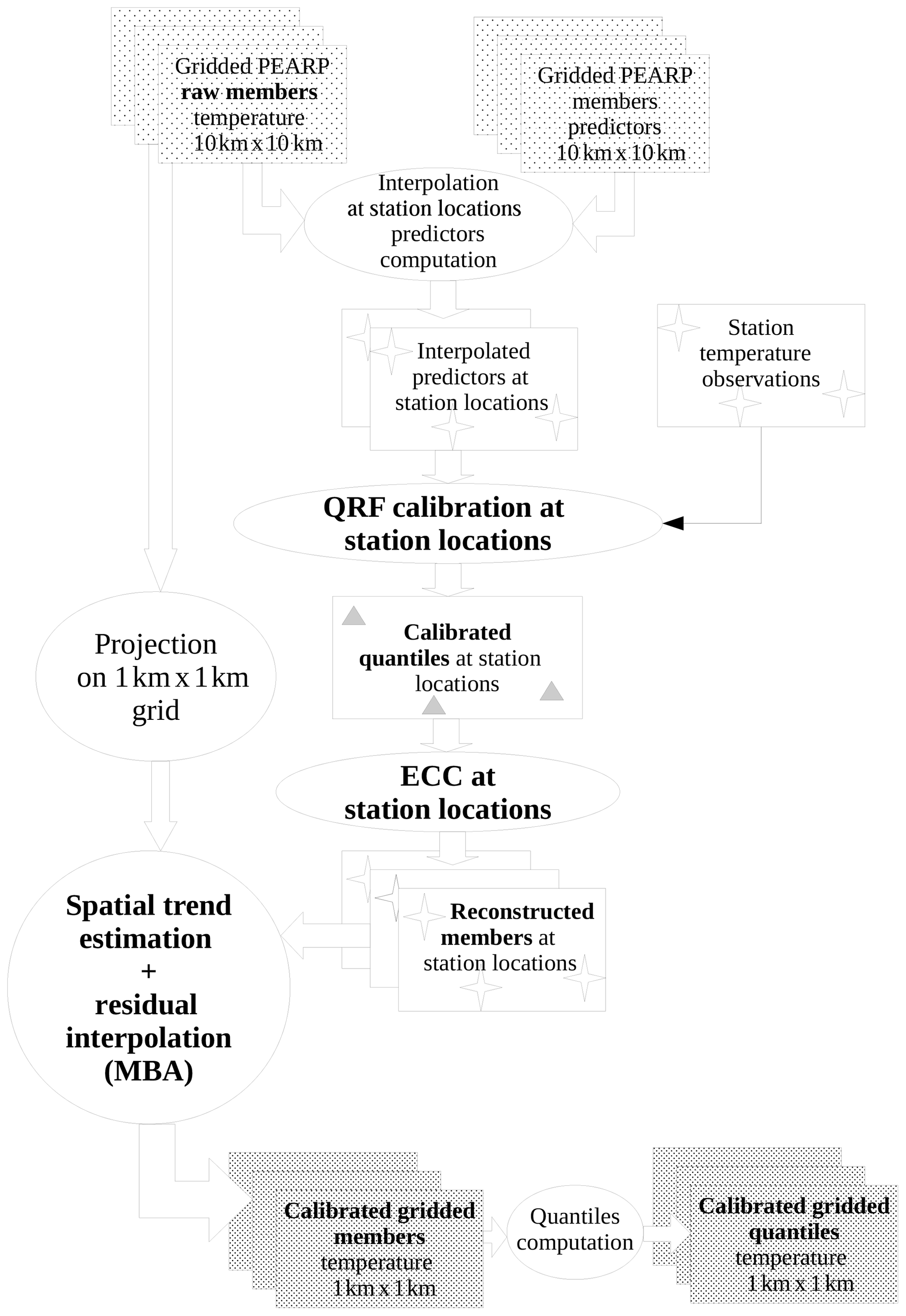
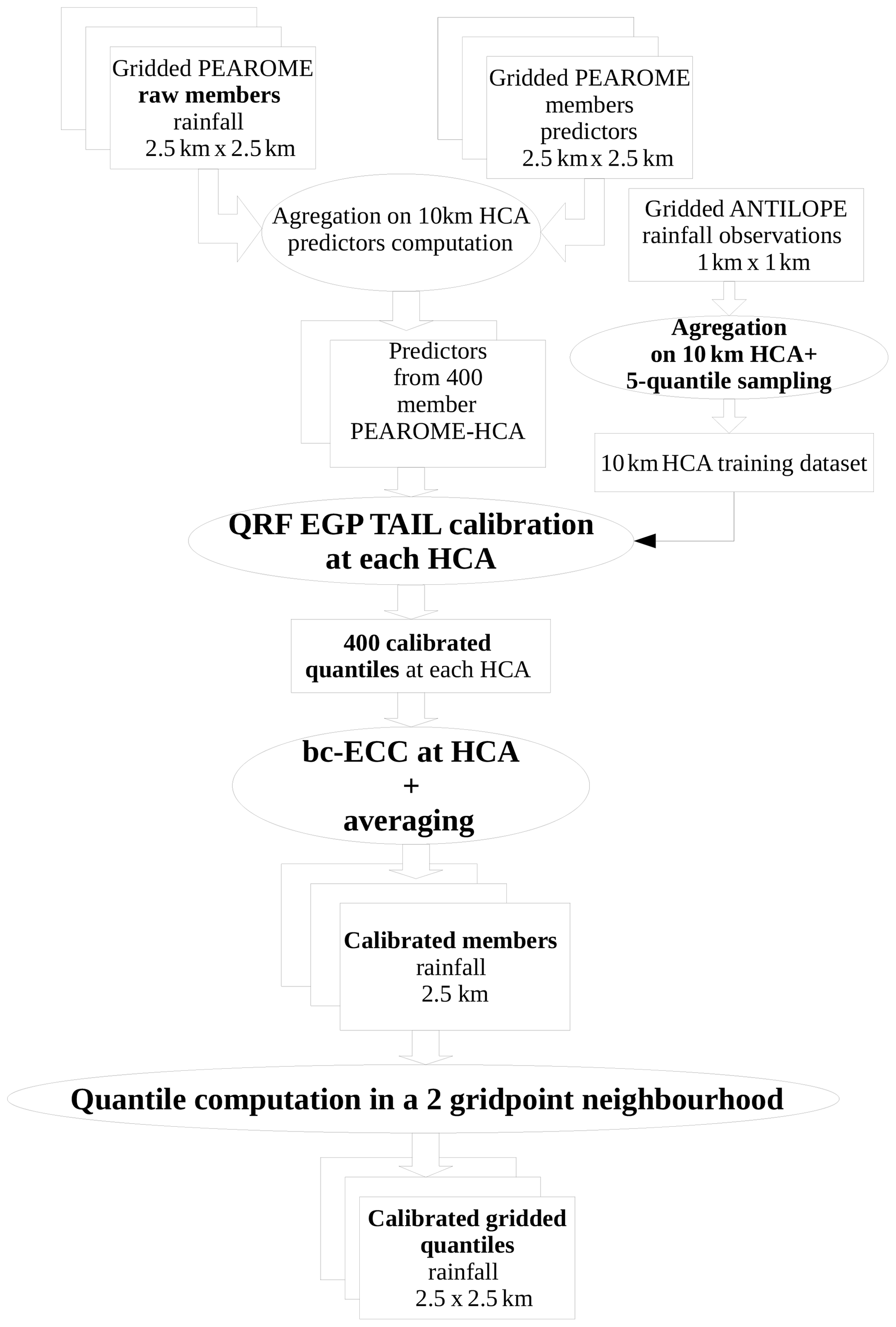
This paper is organized as follows: Sects. 2 and 3 are devoted, respectively, to the complete post-processing chain of surface temperature and hourly rainfall, shown in two flowcharts (Figs. 1 and 2). For each section, a first subsection describes the EPS subject to post-processing and its operational configuration. We also describe the predictors involved in post-processing procedures. The second subsection comprises a short explanation of QRF or the QRF EGP TAIL technique, particularly their adjustments set up for an operational and robust post-processing. The third subsection introduces the post-processing “after post-processing” work: for the post-processing of post-processed temperatures, we exhibit the algorithm of interpolation and downscaling of scattered predictive distributions. For rainfall intensities, a variant of the ECC technique is presented. The last subsection describes the evaluation of post-processing techniques through both global predictive performance and/or a day-to-day case study. A discussion and our conclusions are presented in Sects. 4 and 5.

2 Surface temperature

We present here the French ARPEGE global NWP model, for temperature calibration.

2.1 ARPEGE and ARPEGE EPS

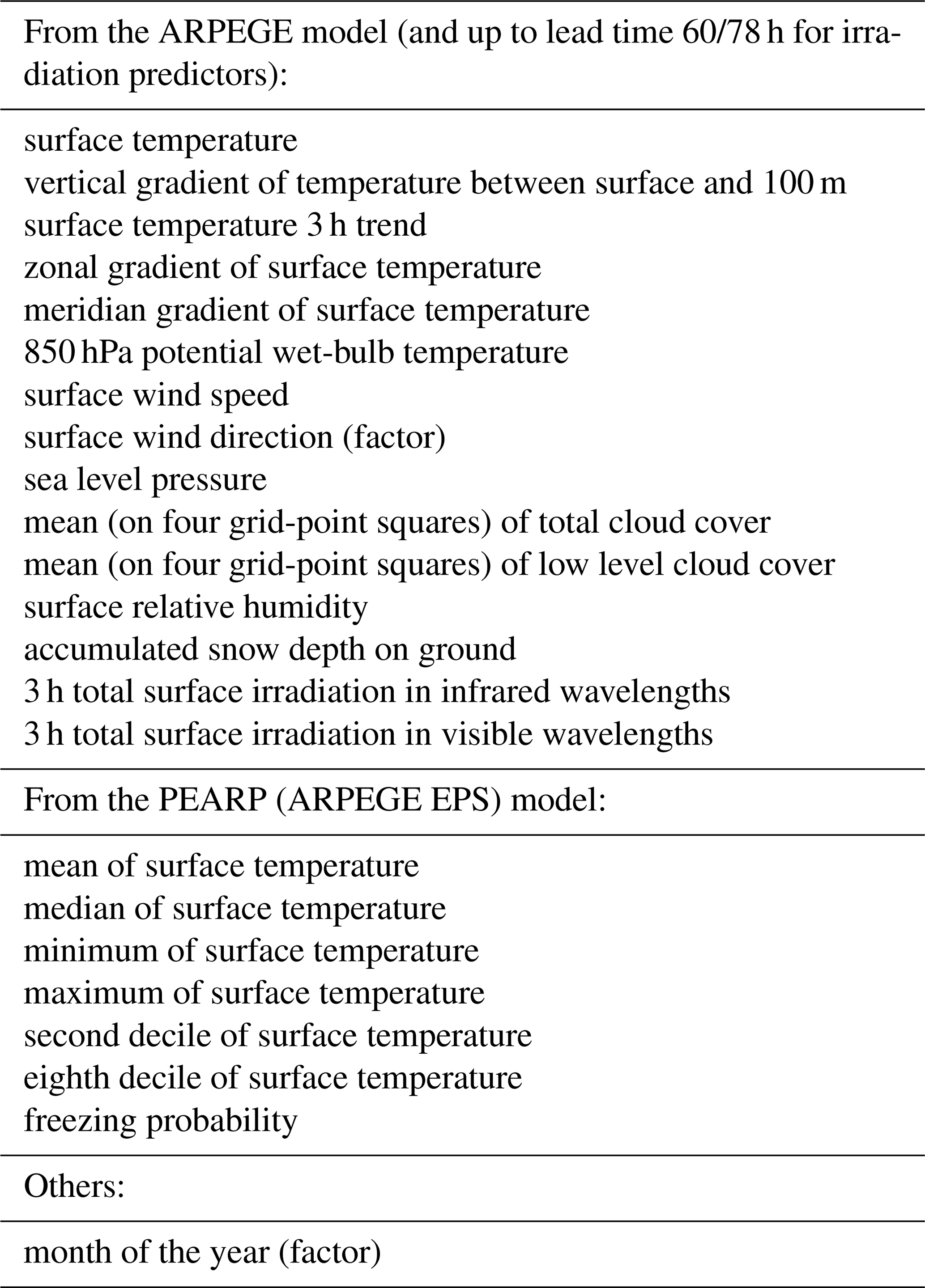
The ARPEGE NWP model (Courtier et al., 1991) has been in use since 1994. Its 35-member EPS, called PEARP, has been in use since 2004, and a complete description is available in Descamps et al. (2015). These global models have been drastically improved throughout the years and their respective grid scale on western Europe is 5 km for ARPEGE and 7.5 km for PEARP; forecasts are made four times per day from 0 to 108 h every 3 h. Calibration is performed on more than 2000 stations across western Europe; see Fig. 3 for the localization of these stations on our target grid (called EURW1S100). The gridded data are bilinearly interpolated on the observation locations. The data span 2 years from 1 September 2015 to 31 August 2017. The variables involved in the calibration algorithm are provided in Table 1. Operational calibration is currently performed for two initializations only (06:00 and 18:00 UTC). Moreover, predictors from the deterministic ARPEGE model are available up to the lead time 60 h (except total surface irradiation predictors, which are available from 60 to 78 h every 6 h).

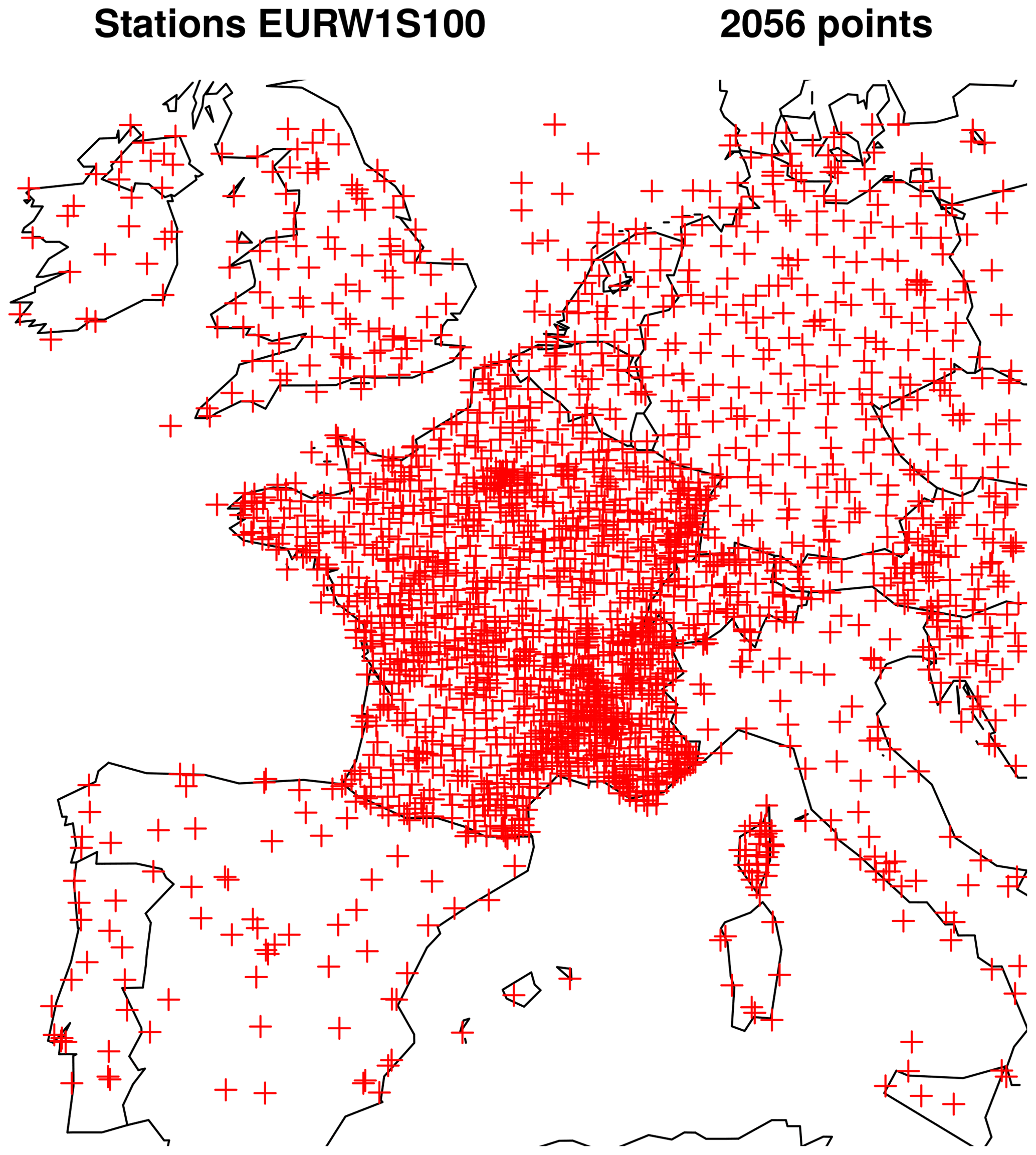
https://www.nonlin-processes-geophys.net/27/329/2020/npg-27-329-2020-f03

Figure 3Localization of stations on the target grid.

Table 1Predictors involved in station-based PEARP post-processing. The target variable is surface temperature.

Download Print Version | Download XLSX

We can assume that this data set is less abundant than in Taillardat et al. (2016). This is mainly due to the number of stations covered and the target grid after interpolation, the kilometric AROME grid in western Europe (EURW1S100), which is composed of more than 4 millon grid points. Since the principle of statistical post-processing is to build a statistical model linking observations and NWP outputs, two strategies can be considered: the first one is to build a gridded observation archive on the target grid, using scattered station data and a spatialization technique, and to estimate statistical models for each grid point or each group of grid points (block-MOS technique, Zamo et al., 2016). But although the block-MOS technique is efficient when dealing with deterministic outputs, preliminary tests (not shown here) are inconclusive regarding post-processing of ensembles. Furthermore, estimating a QRF model for each grid point and lead time is not adapted to the operational use, since it would involve a prohibitive size of constants (around 4 TB in this case) to load and store into memory. The alternative strategy is the following: perform calibration on station data and use a quick spatialization algorithm, very similar in its principle to regression kriging, in order to produce quantiles on the whole grid. The computation of calibrated members involves an ECC phase and the same spatialization algorithm.

2.2 QRF calibration technique

Based on the work of Meinshausen (2006), QRFs rely on building random forests from binary decision trees, in our case the classification and regression trees from Breiman et al. (1984). A tree iteratively partitions the training data into two groups. A split is made according to thresholds for one of the predictors (or according to some set of factors for qualitative predictors) and chosen such that the sum of the variance of the two subgroups is minimized. This procedure is repeated until a stopping criterion is reached. The final group (called “leaf”) contains training observations with similar predictor values. An example of a tree with four leaves is provided at the top of Fig. 4.

Binary decision trees are prone to unstable predictions insofar as small variations in the learning data can result in the generation of a completely different tree. In random forests, Breiman (2001) solves this issue by averaging over many trees elaborated from a bootstrap sample of the training data set. Moreover, each split is determined on a random subset of the predictors.

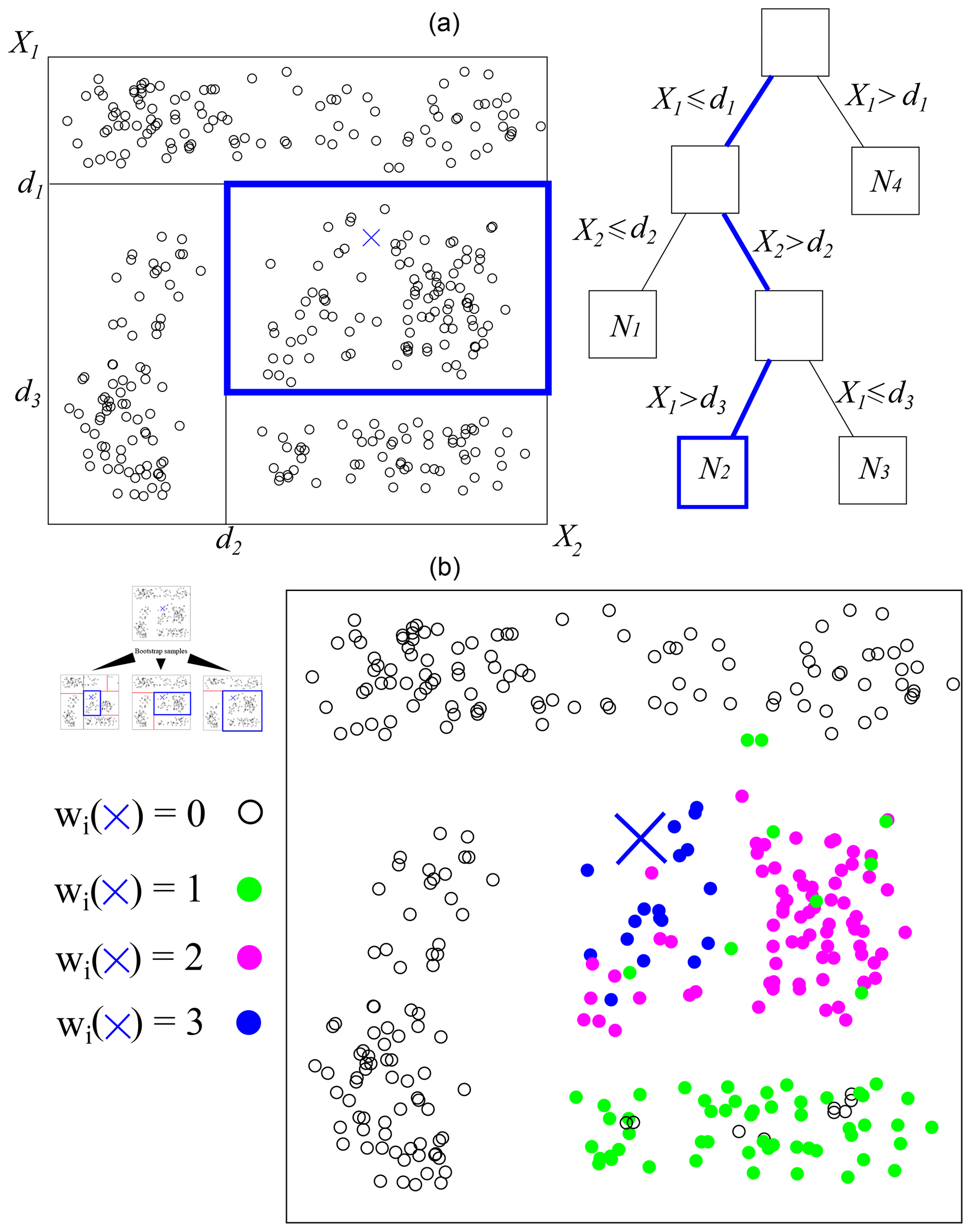
https://www.nonlin-processes-geophys.net/27/329/2020/npg-27-329-2020-f04

Figure 4Two-dimensional example of a (a) binary regression tree and (b) three-tree forest. A binary decision tree is built from a bootstrap sample of the data at hand. Successive dichotomies (lines splitting the plane) are made according to a criterion based on observations’ homogeneity. For a new set of predictors (the blue cross), the path leading to the corresponding observations is followed. The predicted CDF is the aggregation of the results from each tree.

Download

When a new set of predictors x is available (the blue cross in Fig. 4), the conditional cumulative distribution function (CDF) is made by the observations Y_i corresponding to the leaves to which the values of x lead in each tree. The predicted CDF is thus

\begin{matrix} (1) & \hat{F} (y | x) = \sum_{i = 1}^{n} ω_{i} (x) 1 ({Y_{i} \leq y}), \end{matrix}

where the weights ω_i(x) are deduced from the presence of Y_i in a final leaf of each tree when following the path of x.

See, for example, Taillardat et al. (2016, 2019), Rasp and Lerch (2018), and Whan and Schmeits (2018) for detailed explanations and comparisons with other techniques in a post-processing context.

2.3 Operational adjustments for temperature

A direct application of the QRF algorithm for forecasting temperature distribution is suboptimal. Indeed, although QRF is able to return weather-related features such as multi-modalities, alternatives scenarios, and skewed distributions, the method cannot go beyond the range of the data. In the operational chain, the QRF algorithm is not trained with observations but with the errors between the observation and the ensemble forecast mean. The result of Eq. (1) is, in this case, the error distribution before translation around the raw ensemble mean. The predictive distributions are now constrained by the range of errors made by the ensemble mean. This anomaly-QRF approach generates better distributions than QRF for the prediction of cold and heat waves and leads to an improvement of about 7 % (not shown here) in the averaged continuous ranked probability score (CRPS; Gneiting and Raftery, 2007), thanks to this NWP-dependent variable response.

2.4 Ensemble copula coupling

The ensemble copula coupling method (Schefzik et al., 2013) provides spatiotemporal joint distributions derived from the raw ensemble structure. Its small computational cost makes it, for us, the preferred way to reorder calibrated marginal distributions, even if other techniques, such as Schaake shuffle, have their advantages (Clark et al., 2004). Therefore, we make the assumption that on the homogeneity calibration area (HCA), the structure of the raw ensemble is temporally and spatially sound. Recently, Ben Bouallègue et al. (2016) and Scheuerer and Hamill (2018) proposed an improvement of the ECC technique using, respectively, past observations and simulations. In the context of hourly quantities in hydrology, Bellier et al. (2018) show that perturbations added to the raw ensemble lead to satisfactory multivariate scenarios.

2.5 Interpolation of scattered post-processed temperature

2.5.1 Principle

The problem at hand is challenging.

The domain covers a large part of western Europe, from coastal regions to Alpine mountainous regions, subject to various climate conditions (oceanic, Mediterranean, continental, Alpine).
Data density is very inhomogeneous (from the high density of stations over France to the somewhat dense network over the UK, Germany, and Switzerland and the sparse density over Spain and Italy).
Interpolation has to be extremely fast, since more than 1824 high-resolution spatial fields have to be produced in a very short time.

Common methods used to interpolate meteorological variables include inverse distance weighting (IDW; Zimmerman et al., 1999) and thin plate splines (TPS; Franke, 1982) – both considered deterministic methods – and kriging (Cressie, 1988), including kriging with external drift to take topography effects into account (Hudson and Wackernagel, 1994). But while IDW suffers from several shortcomings such as cusps, corners, and flat sports at the data points, preliminary tests showed that both TPS and kriging did not satisfy computation time requirements.

Therefore, a new technique has been developed, very similar to “regression kriging”, based on the following principle: at each station location, perform a regression between post-processed temperatures and raw NWP temperatures, using additional gridded predictors as well. The resulting equation is then applied to the whole grid to produce a spatial trend estimation. Regression residuals at station locations are then interpolated. Spatial trend and interpolated residuals are summed to produce the resulting field. Interpolation of residual fields is performed using an automated multi-level B-spline analysis (MBA; Lee et al., 1997), an extremely fast and efficient algorithm for the interpolation of scattered data.

2.5.2 Spatial trend estimation

Several studies have investigated the complex relationships between topography and meteorological parameters; see e.g. Whiteman (2000) and Barry (2008). A naive model would be a linear decrease in temperatures with altitude, which is not realistic for temperature at the daily or hourly scale, since the vertical profile may be very different from the profile of free air temperature. An important phenomenon, which has often been studied and subject to modelling, is cold air pooling in valleys with the diurnal cycle. Frei (2014) uses a change-point model to describe non-linear behaviour of temperature profiles.

Topographical parameters include altitude, distance to coast and additional parameters computed following the AURELHY method (Bénichou, 1994). The AURELHY method is based on a principal component analysis (PCA) of altitudes. For each point of the target grid, 49 neighbouring grid-point altitudes are selected, forming a vector called a landscape. The matrix of landscapes is processed through a PCA. We determine that this method efficiently summarizes topography, since first principal components can easily be interpreted in terms of peak/depression effect (PC1), northern/southern slopes (PC2), eastern/western slopes (PC3) or “saddle effect” (PC4). These AURELHY parameters are presented in Fig. 5.

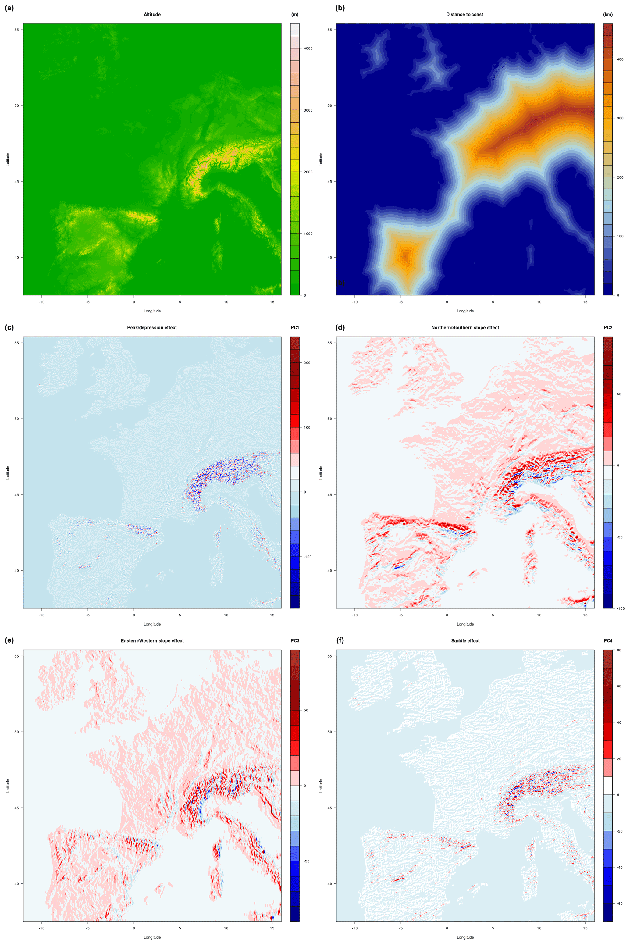
https://www.nonlin-processes-geophys.net/27/329/2020/npg-27-329-2020-f05

Figure 5Altitude (a), distance to sea (b), and PC1 to PC4 (c–f).

For the interpolation of climate data, most of the time only topographic data are available, which may play the role of ancillary data in estimating the spatial trend. In our case, another important source of information is provided by the NWP temperature field at the corresponding lead time for each member. As such, PEARP data may not be directly used, since their resolution is coarser than the target resolution (7.5 km rather than 1 km). Therefore, PEARP data are projected onto the target grid using the following procedure: for each of 7.5 km grid points, a linear transfer function is estimated through a simple linear regression between each of the 100 AROME temperature data points (available on the 1 km resolution grid) and the corresponding ARPEGE data point. Since this relationship is likely to change over seasons and time of day, these regressions are computed seasonally, and for every hour of the day, using 1 year of data. This is a crude but quick way to perform downscaling of PEARP data, as will be shown later.

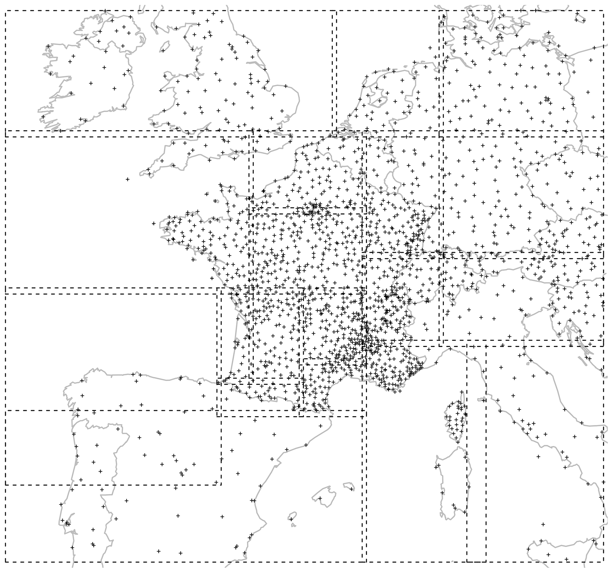
https://www.nonlin-processes-geophys.net/27/329/2020/npg-27-329-2020-f06

Figure 6Domains used for spatialization of post-processed temperatures.

Since interpolation is to be performed on a very large domain, with greatly varying data density, several regressions are computed on smaller sub-domains denoted by D, whose boundaries are given in Fig. 6. Note that the size of the domains depends on the stations' spatial density. Further, domains overlap: at their intersection, spatial trends are averaged, and weights add up to 1 and are a linear function of inverse distance to the domain frontier. This simple algorithm is very efficient in eliminating any discontinuity between adjacent domains that might appear otherwise.

For a given base time b and lead time t, validity time is denoted as v and season is denoted as S.

We denote alti_i (or d2s_i, PC1_i, PC2_i, PC3_i, or PC4_i) values of altitude (or distance to sea, and principal component of elevations 1 to 4) at grid point i of the target grid. For every base time b and lead time t, let T_k be the calibrated temperature forecast of the kth station point of subdomain D, corresponding to grid point i of the target grid (0.01^∘ × 0.01^∘) and grid point j of the PEARP 0.1^∘ × 0.1^∘ grid, and let T_j be the corresponding raw PEARP temperature forecast (same member, base time and lead time as T_k) at grid point j. Then,

\begin{array}{l} (2) & T_{k} & = β_{0_{D}} + β_{1_{D}} (γ_{0_{i} j v S} + γ_{1_{i} j v S} T_{j}) \\ (3) & + β_{2_{D}} {alti}_{i} + β_{3_{D}} ({alti}_{i} - a_{D}^{*}) 1 {{alti}_{i} > a_{D}^{*}} \\ (4) & + β_{4_{D}} d 2 s_{i} \\ (5) & + α_{1_{D}} PC 1_{i} + α_{2_{D}} PC 2_{i} + α_{3_{D}} PC 3_{i} + α_{4_{D}} PC 4_{i} \\ (6) & + ϵ_{k} . \end{array}

Equation (2) corresponds to the linear influence of the linear projection function of T_j on target grid point i. Equation (3) corresponds to the altitude effect, with a possible change in slope of the vertical temperature gradient at altitude $a_{D}^{*}$ , the value of which is tested on a grid of 10 specified elevations for each domain D. Equation (4) is the influence of distance to sea. Equation (5) is related to the first four principal components of elevation landscapes. The last term ϵ_k is the regression residual. The distance to the sea predictor appears only for domains including seashores. Furthermore, domains containing too few station points, namely the Spanish and Italian domains, have only one predictor, which is a linear projection of PEARP temperature data: $γ_{0_{i} j v S} + γ_{1_{i} j v S} T_{j}$ .

The model estimation of parameters $β_{0_{D}}, β_{1_{D}}, β_{2_{D}}, β_{3_{D}}, β_{4_{D}}, α_{1_{D}}, α_{2_{D}}, α_{3_{D}}, α_{4_{D}},$ and $a_{D}^{*}$ is performed by means of ordinary least squares, with the model selection automatically ensured by an Akaike information criterion (AIC) procedure. This model selection is influenced by the weather situation, but the most often selected variables are the linear projection function of T_j and/or the altitude effect – since they are very well correlated. Distance to sea and PC1 may also be selected quite frequently. PC2 to PC4 are selected much less frequently.

2.5.3 Residual interpolation

We aim to use an exact, automatic and fast interpolation method for residual interpolation. Although TPS and kriging may be computed in an automated way, those methods do not meet our criteria in terms of computation time.

While not strictly an exact interpolation method, the MBA algorithm was chosen as it is an extremely fast algorithm. Furthermore, the degree of smoothness and exactness of the method may be precisely controlled, as recalled by Saveliev et al. (2005).

A precise description of this method is beyond the scope of this article. We just briefly recall that the MBA algorithm relies on a uniform bicubic B-spline surface passing through the set of scattered data to be interpolated. This surface is defined by a control lattice containing weights related to B-spline basis functions, the sum of which allows surface approximation. Since there is a tradeoff between smoothness and accuracy of approximation via B splines, MBA takes advantage of a multiresolution algorithm. MBA uses a hierarchy of control lattices, from coarser to finer, to estimate a sequence of B-spline approximations whose sum achieves the expected degree of smoothness and accuracy. Refer to Lee et al. (1997) for a complete description of the algorithm.

During testing, we found out that 13 approximations were sufficient to ensure a quasi-exact interpolation (magnitude of error, around 0.0001 ^∘C at station locations) for a visual rendering extremely similar to interpolation TPS, at the cost of a small and acceptable computing time. The solution with 12 approximations was discarded, as it was not precise enough (magnitude of error around 0.3 ^∘C at station locations), meaning that interpolation could no longer be considered to be exact. When using 14 approximations, computation time dramatically increased.

An important point at the practical level is that the interpolation of residuals is performed only once on the whole grid. We found that undesirable boundary effects could appear at the edges of domains D when residuals were interpolated at each domain D alone.

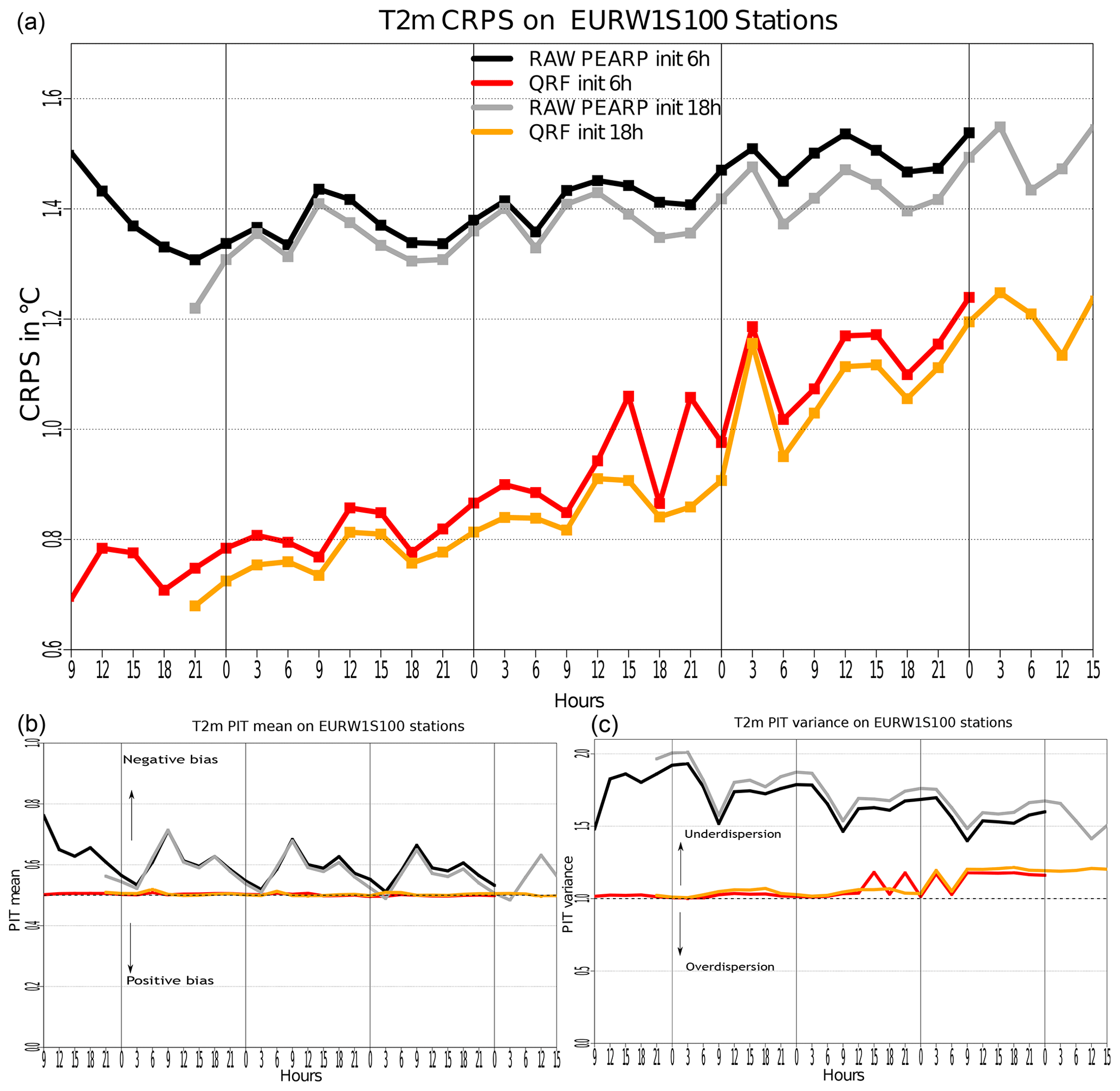
https://www.nonlin-processes-geophys.net/27/329/2020/npg-27-329-2020-f07

Figure 7Results of PEARP post-processing of temperature in the 2056 EURW1S100 stations with average CRPS (a) and mean (b) and variance (c) of the PIT statistic, related to rank histograms. The validation is made by a 2-fold cross-validation on the 2 years of data (one sample per year).

Download

2.6 Results for the temperature post-processing chain

2.6.1 Results of station-wise calibration

We present here the results of the post-processing of PEARP temperature in EURW1S100 stations. The hyperparameters for QRF are derived from Taillardat et al. (2016) but with a smaller number of trees (200). The validation is made by a 2-fold cross-validation on the 2 years of data (one sample per year). For each base and lead time, Fig. 7 shows the averaged CRPS in panel a and the PIT statistic mean and 12× variance in panels b and c. These statistics represent the bias and dispersion of the rank histograms (Gneiting and Katzfuss, 2014; Taillardat et al., 2016). Subject to probabilistic calibration, the mean of the statistic should be 0.5 and the variance 1∕12, which implies the flatness of rank histograms.

The gain in CRPS is obvious after calibration, whatever the base and lead times. Moreover, the hierarchy among base times is maintained. In both panels b and c, post-processed ensembles are unbiased and well dispersed, in contrast to raw ensembles, which exhibit (cold with diurnal cycle) bias and underdispersion. Nevertheless, we notice that post-processed distributions show a slight underdispersion at the end of lead times. This is due to the absence of predictors coming from the deterministic ARPEGE model. These predictors do not relate directly to temperature, and thus the addition of weather-related predictors is crucial here for uncertainty accounting. We believe that radiation predictors are most important here, since the presence or absence of these predictors is linked to the “roller coaster” behaviour of post-processed PIT dispersion around a 3 d lead time.

2.6.2 Performance of interpolation algorithm

Prior to any use in the spatialization of post-processed PEARP fields, performances of the interpolation method were evaluated for deterministic forecasts.

This paragraph is devoted to the evaluation of an earlier version of the current spatialization algorithm over France, which differs only in the fact that NWP temperature fields are not available in the predictor set for spatial trend estimation. Benchmarking data consist of 100 forecasts. For each date, 20 cross-validation samples are randomly generated, removing 40 points from the full set of points. Original forecast values and interpolated forecast values are then compared, and standard scores (bias, root mean square error, mean absolute error, 0.95 quantile of absolute error) are computed. Scores are then compared to the COSYPROD interpolation scheme, the previous operational interpolation method. COSYPROD is a quick interpolation scheme which predates both the first and current versions of our algorithm, adapted to interpolation at a set of some production points and derived from the IDW method.

Results show that, regardless of the method, bias remains low, but the new spatialization method outperforms COSYPROD in terms of root mean square error, mean absolute error, and 0.95 quantile of absolute error (Fig. 8).

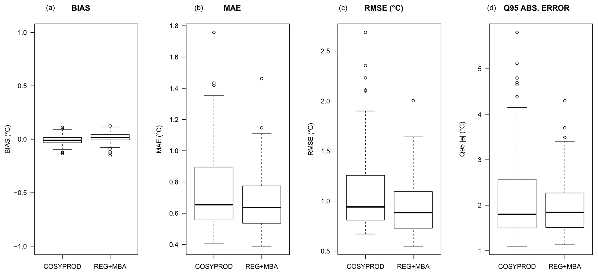
https://www.nonlin-processes-geophys.net/27/329/2020/npg-27-329-2020-f08

Figure 8Boxplots of bias (a), mean absolute error (b), root mean square error (c) and 0.95 quantile of absolute error (d) for COSYPROD (left boxplot) and the new method (right boxplot).

Download

Additionally, the described spatialization procedure has already been used operationally for the interpolation of deterministic temperature forecasts since May 2018. In this application, its performances were evaluated routinely over a large set of climatological station data, which only measure extreme temperatures and do not provide real-time data. Hence, this data set is discarded from any post-processing, but may serve as an independent data set for validation. When comparing forecast performances related to this data set, the increase in root mean square error is around 0.3 ^∘C compared to forecast errors estimated at post-processed station data. Hence, this extra 0.3 ^∘C root mean square error may be considered an error due to the interpolation process. Note that this is much lower than what was estimated during the cross-validation phase: all in all, forecast errors and interpolation errors are not added together, but compensate each other to some extent.

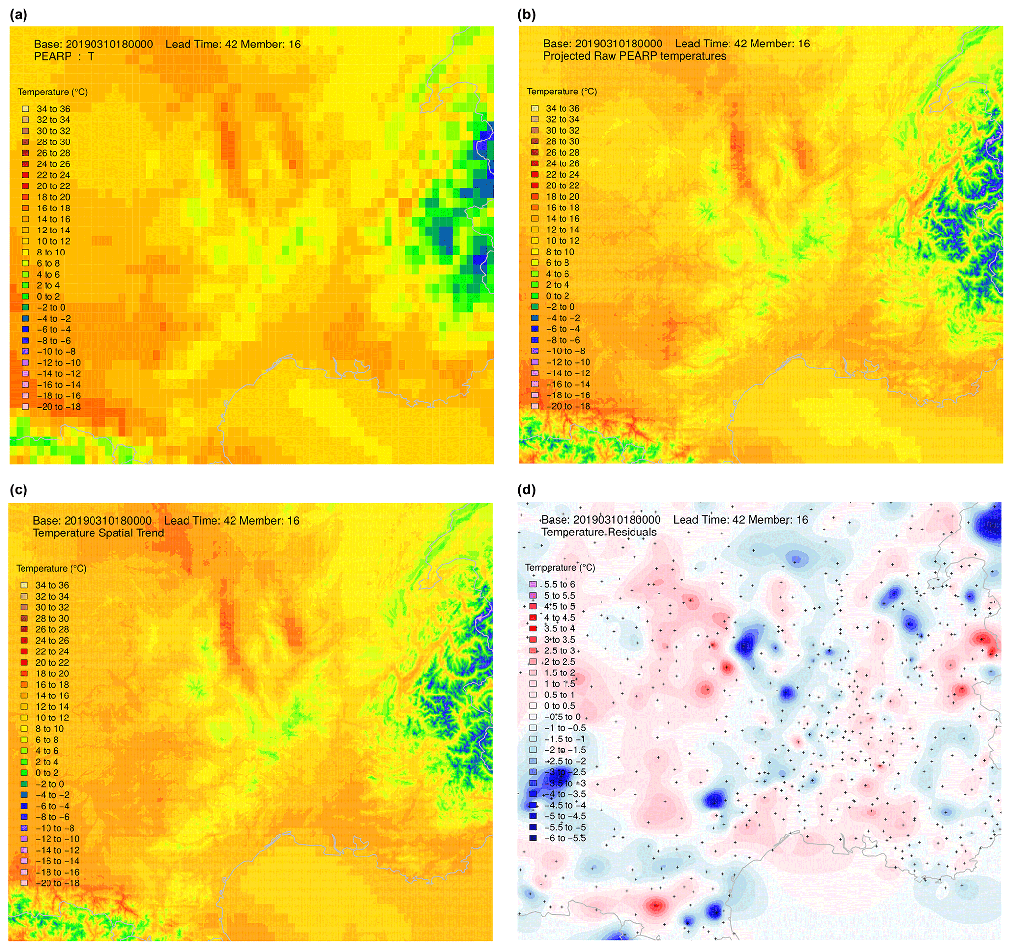
https://www.nonlin-processes-geophys.net/27/329/2020/npg-27-329-2020-f09

Figure 9Step-by-step procedure illustrated over the south-east of France: raw member temperatures on a 7.5 km grid (a), raw projected temperatures on a 1 km grid (b), spatial trend estimation using a regression model on subdomains (c), and field of residuals interpolated using a MBA procedure with 13 layers of approximation (d).

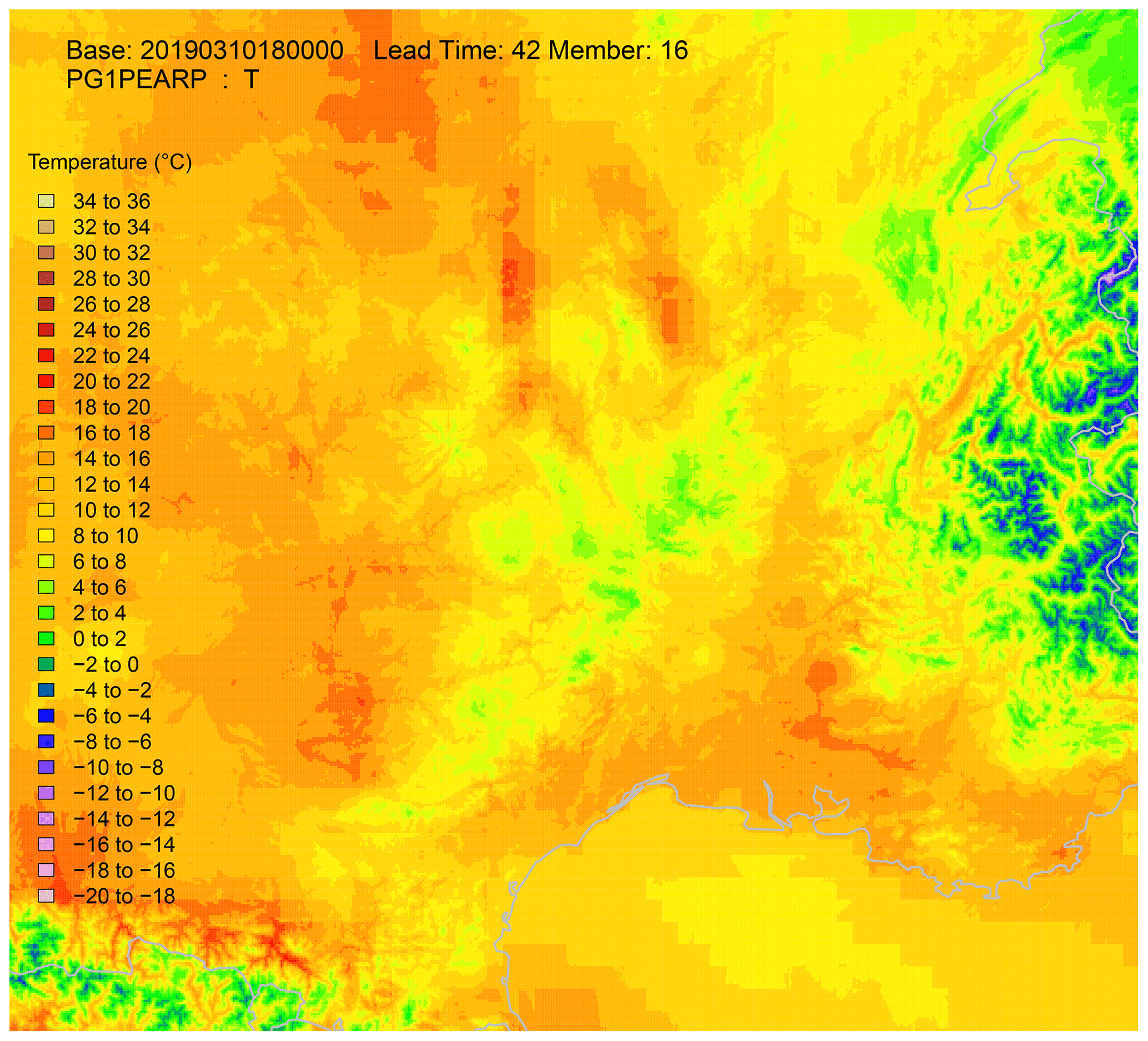
https://www.nonlin-processes-geophys.net/27/329/2020/npg-27-329-2020-f10

Figure 10Resulting field over the south-east of France.

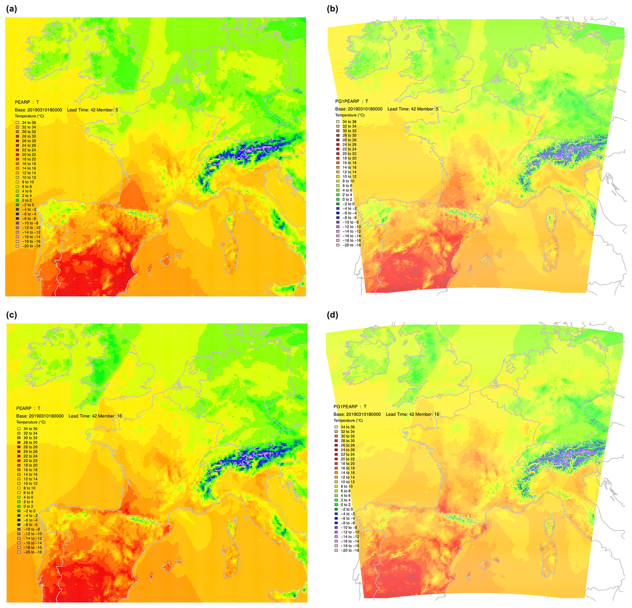
https://www.nonlin-processes-geophys.net/27/329/2020/npg-27-329-2020-f11

Figure 11Raw PEARP member 6 temperature field (a) and the same after calibration, ECC and interpolation phase (b) together with raw (c) and post-processed temperature fields (d) for member 16. Note that the whole procedure can only be applied to the AROME domain.

An illustration of the whole procedure is illustrated on PEARP temperatures of base time 3 October 2019, 18:00 UTC, for lead time 42 h. The temperature field of raw member 16 is presented in Fig. 9, together with the same field projected onto the EURW1S100 grid. The estimated spatial trend is also shown, and residuals interpolated using the MBA procedure with 13 approximation layers can also be found in Fig. 9. The resulting field, after calibration, ECC, and spatial interpolation phases is presented in Fig. 10. The same process is repeated here for member 6 (Fig. 11).

Note that during the full processing, field values were modified during the calibration process. But ECC and interpolation are able to maintain the main features of the original field; i.e. it is the passage of a front, which is not situated in the same location for both members.

3 Hourly rainfall

We present the high-resolution limited model area NWP model AROME, for the post-processing of hourly rainfall.

3.1 AROME and AROME EPS

The AROME non-hydrostatic NWP model (Seity et al., 2011) has been in use since 2007 in the limited area of Fig. 3. The associated 16-member EPS, called PEAROME (Bouttier et al., 2016), has been in operational use since the end of 2016. The deterministic model operates on the 1 km EURW1S100 grid, whereas PEAROME runs on a 2.5 km grid. Forecasts are made four times a day from 0 to 54 h. Data span 2 years from 1 December 2016 to 31 December 2018. Calibration is not performed on the 2.5 km grid, but on a 10 km grid. Thus we consider PEAROME here as a $16 \times 5 \times 5 = 400$ -member pseudo-ensemble on a 10 km grid. We do this for three reasons.

We reduce spatial penalty issues due to the high resolution of the raw EPS (see e.g. Stein and Stoop, 2019).
We improve ensemble sampling and, we hope, the quality of predictors.
We reduce computational costs by a factor 25.

The post-processing is conducted on these 10 km HCA grid points using ANTILOPE (Laurantin, 2008), the 1 km gridded French radar data set calibrated with rain gauges. Predictors involved in the calibration algorithm are listed in Table 2. Note that the temporal penalties due to the high resolution are considered in this choice of predictors. Operational calibration is currently performed for two initializations only (09:00 and 21:00 UTC) and for lead times up to 45 h.

Table 2Predictors involved in HCA-based PEAROME post-processing. The target variable is hourly rainfall.

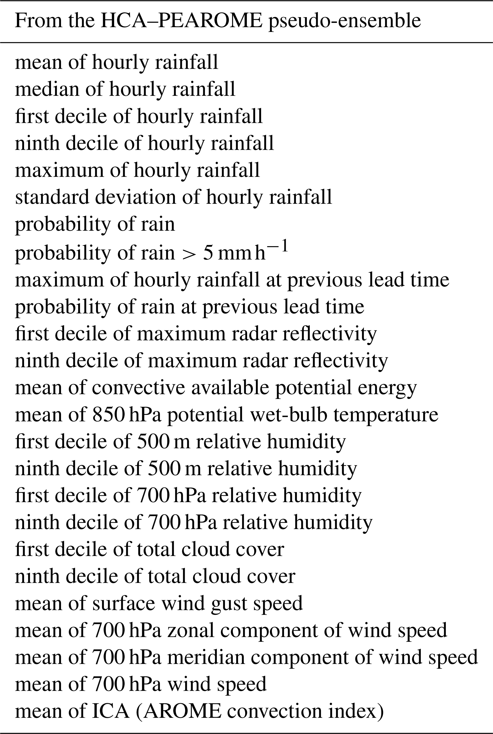
Download Print Version | Download XLSX

The number of predictors is less abundant here than in Taillardat et al. (2019). This number was reduced to 25 due to operational constraints on model size. These predictors were chosen after a variable selection step using VSURF (Genuer et al., 2015) and R (R Core Team, 2015) package randomForestExplainer (Paluszynska, 2017) among more than 50 potential predictors. A complete description of the variable selection is beyond the scope of the paper. To summarize, the most important variables are, on average, minimal and maximal rainfall intensities. These variables are followed by “synoptic” variables such as wind or humidity at medium-level and potential wet-bulb temperature. ICA is roughly the product of the modified Jefferson index (Peppier, 1988) with a maximum between 950 hPa convergence and maximal vertical velocity between 400 and 600 hPa. This latter variable and other variables representing the shape of the raw distribution of precipitation are less decisive on average. Variables not retained in the selection procedure are redundant with the main predictors, such as other convection indices, medium-level geopotential, and low-level cloud cover and surface variables. For each of the 13 900 HCAs, the quantile regression algorithm gives 400 quantiles, attributed to each member of each grid point of the HCA after a derivation of the ECC technique. The values of grid points and members overlapping two or more HCAs are averaged.

3.2 QRF EGP TAIL calibration technique

Note in Eq. (1) that the QRF method cannot predict values outside the range of the training observations. For applications focusing on extreme or rare events, it could be a strong limitation if the data depth is small. To circumvent this QRF feature, Taillardat et al. (2019) propose to fit a parametric CDF to the observations in the terminal leaves rather than using the empirical CDF in Eq. (1). The parametric CDF chosen for this work is the EGPD3 in Papastathopoulos and Tawn (2013), which is an extension of the Pareto distribution. Naveau et al. (2016) show the ability of this distribution to represent low, medium and heavy rainfall and its flexibility. Thus, the QRF EGP TAIL predictive distribution is

\begin{matrix} (7) & G (y | x) = P_{0} + (1 - P_{0}) {[1 - {(1 + \frac{ξ y}{σ})}^{- \frac{1}{ξ}}]}^{κ}, \end{matrix}

where P₀ is the probability of no rain in the QRF output: $\hat{F} (y = 0 | x)$ . The parameters $(κ, σ, ξ)$ in Eq. (7) are estimated via a robust method-of-moment (Hosking et al., 1985) estimation.

3.3 Operational adjustments for hourly rainfall

The anomaly-based QRF approach is not employed for hourly rainfall. We believe that the choice of a centering variable is as difficult as choosing a good parametric distribution for predictive distributions. In the case of hourly rainfall, the adjustments are not relative to the method, but rather the construction of the training data.

For each HCA, we consider predictors calculated with the 400-member pseudo-ensemble. For each HCA of size 10 km×10 km, 100 ANTILOPE observations are available. We can consider the observation data to come from a distribution. Practically speaking, instead of having one observation Y_i for each set of predictors, in our case we have $(Y_{i_{0}}, Y_{i_{25}}, Y_{i_{50}}, Y_{i_{75}}, Y_{i_{100}})$ , corresponding to the empirical quantiles of order $0, 0.25, 0.5, 0.75, 1$ of ANTILOPE distribution in the HCA. The length of the training sample is inflated by a factor 5, which allows us to take advantage of all the information available instead of upscaling high-resolution observation data.

3.4 ECC for rainfall intensities

As already observed by Scheuerer and Hamill (2018) and Bellier et al. (2017), ECC has innate issues with an undispersed ensemble and, more precisely, the attribution precipitation to zero raw members (i.e. if the calibrated rain probability $\overline{P_{0}}$ is greater than the raw one $\overline{F_{0}}$ ).

In our case, 400 values have to be attributed to the 16 members of the 25 grid points of the HCA. The procedure, called bootstrapped-constrained ECC (bc-ECC), is as follows.

If $\overline{F_{0}} > \overline{P_{0}}$ , a simple ECC is performed.
If not, we perform ECC many times (here 250 times per HCA) and average values.
Then, a raw zero becomes a non-zero only if there is a raw non-zero in a 3 raw grid-point neighbourhood.

In this case, b=250 and c=3. Table 3 gives an example of an HCA of three grid points and two members.

Table 3Example of bc-ECC (b=∞, c=1) for a two-member (M) ensemble in a three-grid-point (gP) linear HCA.

Download Print Version | Download XLSX

As a result, in a member, post-processing can introduce rain in a grid box that is dry in a raw member only if there is a grid point with rain close by in the raw member. This approach ensures coherent scenarios between post-processed rainfall fields and raw cloud cover fields, for example.

3.5 General results and day-to-day examples for rainfall

3.5.1 Hourly rainfall calibration

Due to the high amount of data to process for evaluation (around 200 GB), scores are presented with an averaged lead time and for the base time 09:00 UTC only. More precisely, for each lead time evaluation is made of 400 HCAs over 13 900 HCAs. More than 920 sets of hyperparameters for QRF EGP TAIL were tried, and the numbers retained are 1000 for the number of trees, 2 for the predictors to try and 10 for the minimal node size. In order to make the comparison as fair as possible, the predictive distributions are considered on HCAs and the observation is viewed as a distribution (like in Sect. 3.2.2). As a consequence, the divergence of the CRPS should be used, but the computation of the CRPS on the observations is equivalent (Salazar et al., 2011; Thorarinsdottir et al., 2013). The validation is made by a 2-fold cross-validation on the 2 years of data (one sample per year).

The averaged CRPS between the raw and post-processed ensembles is improved by approximately 30 % (from 0.118 to 0.079).

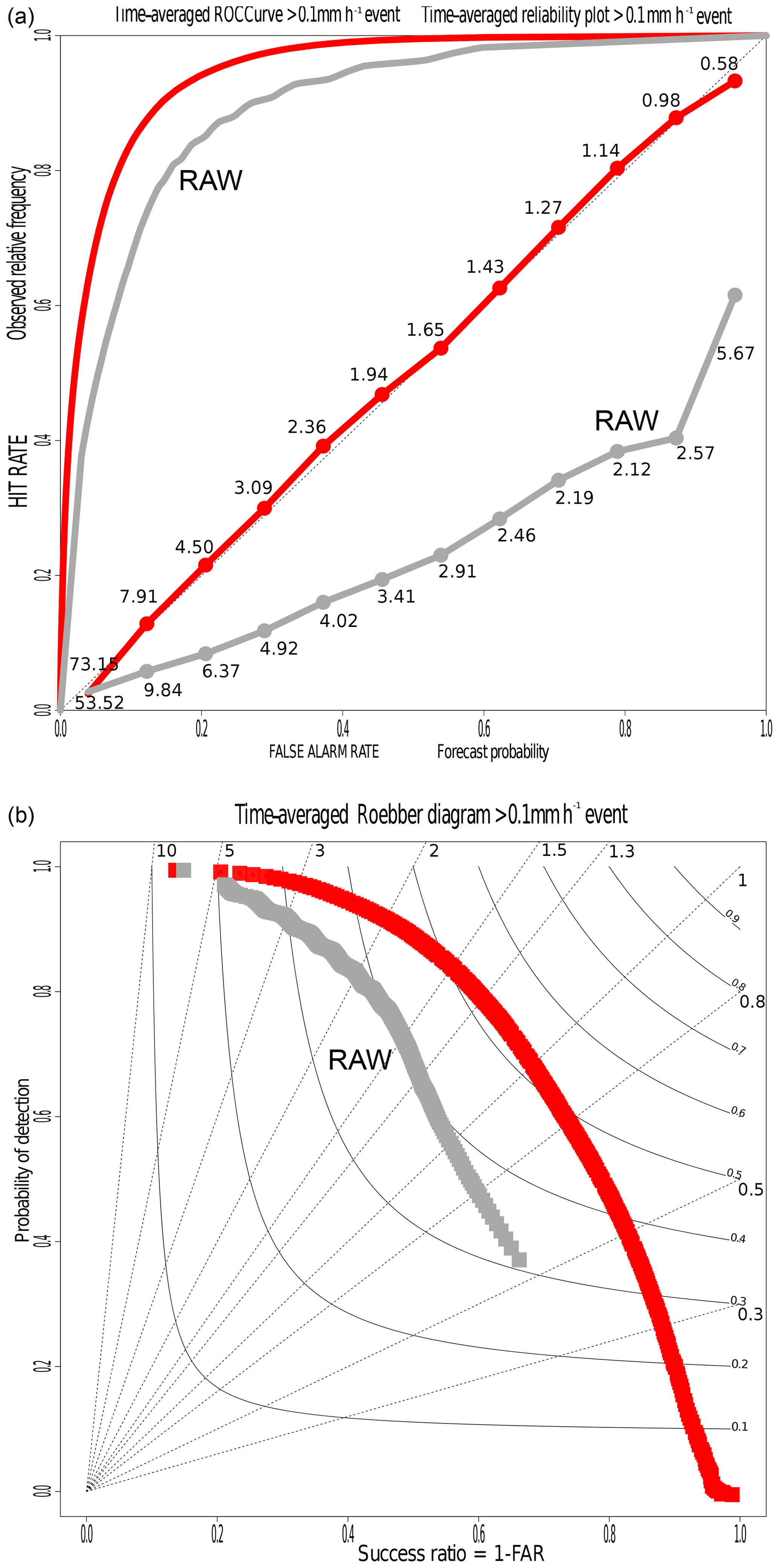
https://www.nonlin-processes-geophys.net/27/329/2020/npg-27-329-2020-f12

Figure 12Receiver operating characteristic (ROC) curve and reliability diagram (a) and categorical performance diagram (b) for the rain event. In the performance diagram, the background lines represent the frequency bias index and the curves represent the critical success index. The raw ensemble suffers from overprediction. The validation is made by a 2-fold cross-validation on the 2 years of data (one sample per year).

Download

Figure 12 focuses on the rain event (more than 0.1 mm h⁻¹). Panel a shows an ROC curve and a reliability diagram in the same plot. Post-processing improves both the resolution and reliability of predictive distributions for the rain event, overpredicted by the raw ensemble. Overprediction of the raw ensemble is also exhibited in the performance diagram (Roebber, 2009) in panel b. Indeed, there is an asymmetry with the top left corner, where frequency bias is more important. Like the ROC curve, the curve in the performance diagram is computed for each quantile of the forecast. The critical success index is increased by 15 %, which means that the ratio of rain events (predicted and/or observed) forecast well is improved by 15 %. Moreover, we can assume here that the minimum (quantile 1/401) of the post-processed distributions nearly never forecasts rain occurrence, but when it does, a false alarm is never made. The minimum (quantile 1/401) of the raw ensemble detects rain occurrence around 40 times out of 100, but when it does, the forecast is wrong around 35 times out of 100 (1− success ratio).

As for increased precipitation, the focus is placed on forecast value. Figure 13 depicts the maximum of the Peirce skill score (PSS; Manzato, 2007) for hourly accumulation thresholds. The maximum of the PSS, which corresponds to the nearest point of the top left corner in ROC curves, is a good way to summarize forecast value (Taillardat et al., 2019). More precisely, most of this improvement is due to the improvement of the hit rate.

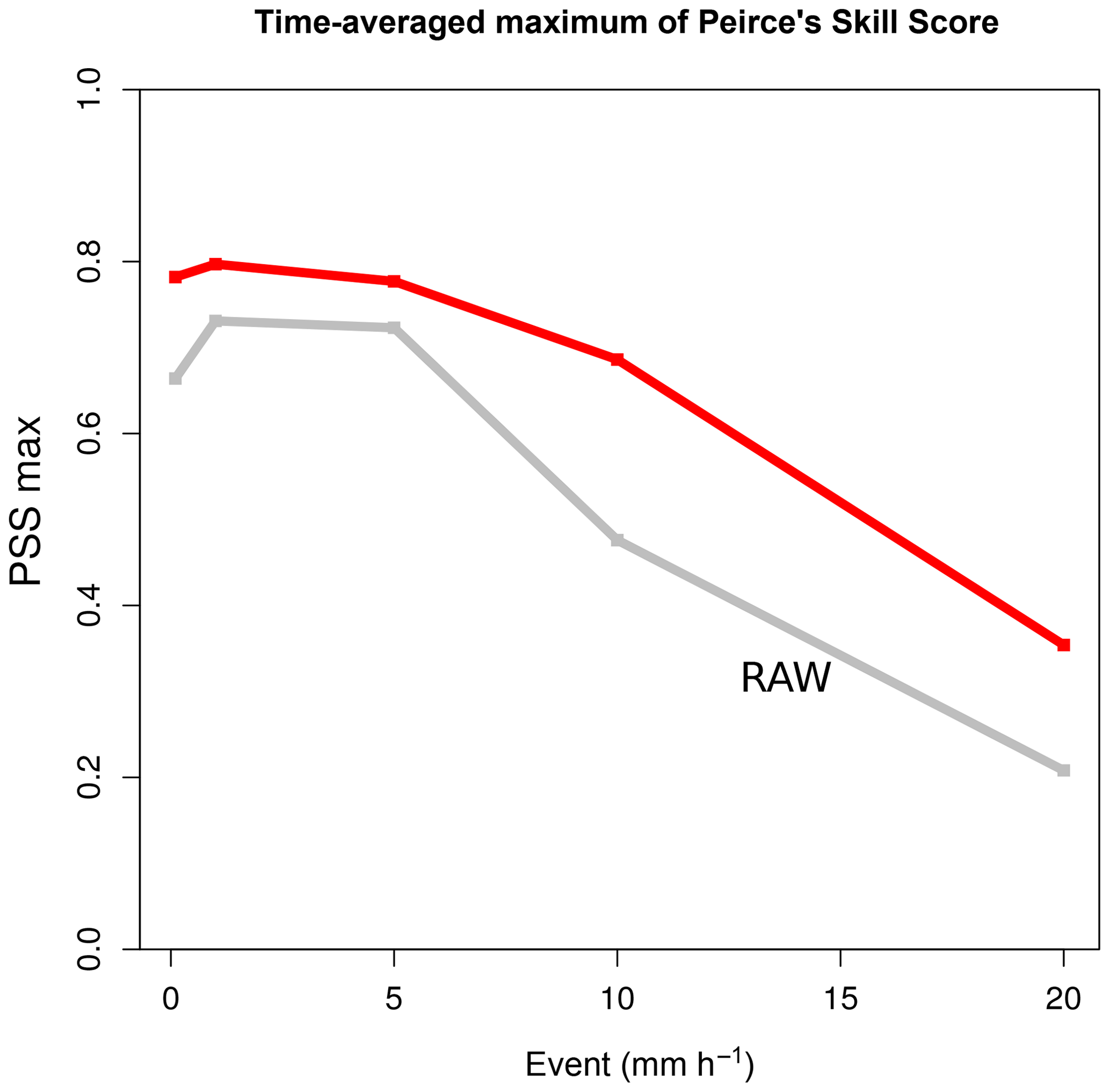
https://www.nonlin-processes-geophys.net/27/329/2020/npg-27-329-2020-f13

Figure 13Maximum of the Peirce skill score among thresholds; the improvement is mainly due to the improvement of the hit rate. The validation is made by a 2-fold cross-validation on the 2 years of data (one sample per year).

Download

https://www.nonlin-processes-geophys.net/27/329/2020/npg-27-329-2020-f14

Figure 14CRPS of daily distributions during October 2019.

Download

3.5.2 Effects on daily rainfall intensities

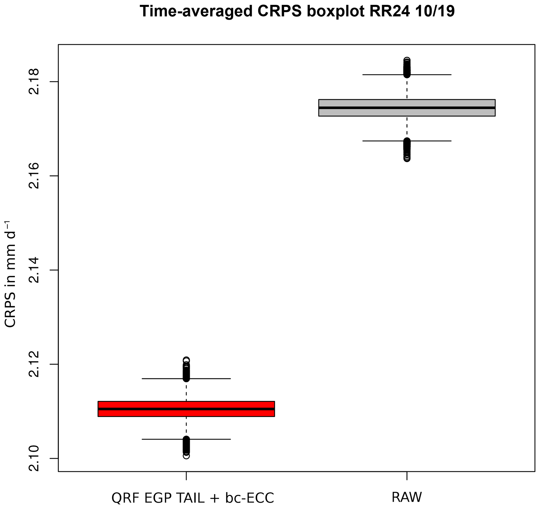
Daily rainfall in between raw and post-processed ensembles was compared in the pre-operational chain during October 2019. In Fig. 14, the CRPS of daily distributions shows that bc-ECC does not deteriorate predictive quality. If we divide by 24, we do not obtain the same results as for raw hourly CRPS, because time penalties disappear with temporal aggregation of hourly quantities. The bc-ECC method does not solve temporal penalties. Therefore, it is not surprising that the daily post-processed CRPS is roughly 24 times the averaged hourly one. Due to the nature of daily precipitation distribution compared to hourly ones (fewer zeros, smaller variance and lighter tail behaviour), we believe that direct post-processing of daily precipitation is more effective if the target variable is daily precipitation.

https://www.nonlin-processes-geophys.net/27/329/2020/npg-27-329-2020-f15

Figure 15Illustration of a heavy precipitation event. On the left, rainfall accumulated on 22 October 2019, with peaks over 300 mm. On the right, quantiles of order 0.1, 0.5, and 0.9 of post-processed (on top) and raw (on bottom) daily rainfall distributions (right maps' data © Google 2019).

We then seek to determine whether calibrated hourly intensities lead to unrealistic or worse daily rainfall intensities than the raw ensemble. In other words, does the bc-ECC generate coherent scenarios? First, in Fig. 15 we show the comparison of the predictive quantiles of daily post-processed (after bc-ECC) and raw intensities. The date is 22 October 2019 and related to a heavy precipitation event in the south of France; 24 h observed accumulations (left of the figure) reach 300 mm. On the right, the quantiles of order 0.1, 0.5, and 0.9 of the post-processed ensemble (top right) and raw ensemble (bottom right) are presented. For this event of interest, we see that bc-ECC does not create unrealistic quantities.

4 Discussion

The two applications described in this article (PEARP temperature and PEAROME rainfall post-processing) are extremely computationally demanding and therefore could not be run on standard workstations within an acceptable timeframe. While codes are implemented on Météo-France's supercomputer, a crucial optimization phase must still be achieved, as two problems had to be solved during the implementation phase.

The very large number of high-resolution fields required, since for each lead time, not only statistical fields (quantiles, mean, standard deviation fields), but also calibrated member fields are computed. This was achieved using inexpensive but efficient methods, such as ECC and MBA, and a massive parallelization of operations, thanks to R High Performance Computing capabilities. The operational code relies on parallel, foreach, DoSNOW, and DoMC packages that enable OpenMP multicore and MPI multinode capabilities. The number of cores used in each node is driven by memory occupation of each process. For example, PEARP temperature uses 4 HPC nodes in 25 min (QRF calibration: 64 cores on 4 nodes (16 cores per node) during 10 min, ECC phase: 12 cores on 1 node during 2 min, spatialization phase: 76 cores on 4 nodes during 15 min). PEAROME rainfall uses 162 cores on 18 HPC nodes during 22 min for QRF EGP TAIL calibration and 432 cores on 6 HPC nodes during 3 min for bc-ECC.
The huge size of objects produced by quantile regression forests. For a given base time, PEARP temperature application requires around 300 GB of data to be read and loaded into memory, while PEAROME rainfall forests represent more than 600 GB of data. Reading this huge amount of data in a reasonable time is possible primarily due to the Infiniband network implemented in the supercomputer, which features a very high throughput and very low latency in I/O operations. Also, stripping R QRF objects from useless features (regarding prediction) allows us to save a substantial amount of space.

Those two applications now deliver post-processed fields of higher quality than raw NWP fields and will be used in the future Météo-France automatic production chain, which is currently in its implementation phase. Post-processed fields are also of higher predictive value and can lead to great benefits for (trained) human forecasters provided that the dialogue between NWP scientists, statisticians and users is strengthened (Fundel et al., 2019).

5 Conclusion

In this article, we show that machine learning techniques allow a very large improvement of probabilistic temperature forecasts – a well-known result that can also be achieved with simpler methods such as EMOS. But while EMOS outputs follow simple and fixed parametric distributions, QRF produces distributions that may preserve the richness of the initial ensemble. Also, a simple method such as ECC coupled with our spatialization algorithm is able to restore realistic high-resolution temperature fields for each member.

Moreover, HCA-based QRF calibration is able to calibrate efficiently a much trickier parameter such as hourly rainfall accumulation – for which the signal for extremes is of special importance and provides realistic rainfall patterns that match initial members.

In the context of forecast automation, it is important to identify the end users and their expectations in order to choose a method that balances complexity and efficiency. In the same vein, minimizing an expected score may be less important than reducing big (and costly) mistakes. For example, the European Center for Medium-Range Weather Forecasts (ECMWF) recently added the frequency of large errors in ensemble forecasts of surface temperature as a new headline score (Haiden et al., 2019).

Of course, applicability of those methods is not restricted to temperature and rainfall. For any parameter that can be interpolated rather easily (humidity for example), our “temperature scheme”, that is, calibration on station locations, ECC and spatialization may be applied. This approach is much less greedy in terms of computation time and disk storage. In addition, Feldmann et al. (2019) show the benefit of using observations rather than gridded analyses. For other parameters, such as cloud cover and wind speed, adaptations of HCA-based calibration (where the observation can also be viewed as a distribution) would be a better option.

The only limitations of post-processing are the availability of good gridded observations or a sufficiently dense station network, and the existence of relevant predictors produced by NWP. Those conditions may not yet always be fully achieved for parameters that remain challenging, such as visibility, for example.

Finally, as recalled in the discussion, production of high-resolution post-processed fields with such techniques has proven to be extremely demanding in terms of CPU and disk storage. Moving the post-processing chain to supercomputers is a challenging but fruitful investment: the learning phase that could take weeks is now achieved in a few hours. This provides extra possibilities for tuning parameters of powerful or promising statistical methods; as mentioned in Rasp and Lerch (2018), this is unavoidable for a quick operational production. Note that using the operational supercomputer hardly interferes with NWP production: by definition, post-processing comes after NWP runs are completed, and the number of nodes required by post-processing is 2 orders of magnitude smaller.

Data availability

The research data come from the operational archive of Météo-France, which is free of charge for teaching and research purposes. Due to its size, we cannot deposit the data in a public data repository. You can find the open data services at https://donneespubliques.meteofrance.fr/ (last access: 28 May 2020).

Supplement

The supplement related to this article is available online at: https://doi.org/10.5194/npg-27-329-2020-supplement.

Author contributions

MT developed the station-wise post-processing of PEARP and the post-processing of PEAROME with bc-ECC. OM developed algorithms of interpolation of scattered data and ECC for temperatures. OM configured the operational chain for temperature. OM and MT currently configure the operational chain for rainfall. OM made figures for temperature. MT created the figures for rainfall and scores. OM and MT wrote the publication, each rereading the other's part.

Competing interests

Maxime Taillardat is one of the editors of the special issue.

Special issue statement

This article is part of the special issue “Advances in post-processing and blending of deterministic and ensemble forecasts”. It is not associated with a conference.

Acknowledgements

The authors would thank the COMPAS/DOP team of Météo-France, and more particularly Harold Petithomme and Michaël Zamo for their work on R codes. The authors would also like to thank Denis Ferriol for his help during the set-up of R codes on the supercomputer.

Review statement

This paper was edited by Sebastian Lerch and reviewed by Jonas Bhend and one anonymous referee.

References

Athey, S., Tibshirani, J., and Wager, S.: Generalized random forests, Ann. Stat., 47, 1148–1178, 2019. a

Baran, S. and Lerch, S.: Combining predictive distributions for the statistical post-processing of ensemble forecasts, Int. J. Forecast., 34, 477–496, 2018. a

Barry, R. G.: Mountain weather and climate, London and New York, Routledge, 2nd edn., 2008. a

Bellier, J., Bontron, G., and Zin, I.: Using meteorological analogues for reordering postprocessed precipitation ensembles in hydrological forecasting, Water Resour. Res., 53, 10085–10107, 2017. a

Bellier, J., Zin, I., and Bontron, G.: Generating Coherent Ensemble Forecasts After Hydrological Postprocessing: Adaptations of ECC-Based Methods, Water Resour. Res., 54, 5741–5762, 2018. a

Ben Bouallègue, Z., Heppelmann, T., Theis, S. E., and Pinson, P.: Generation of scenarios from calibrated ensemble forecasts with a dual-ensemble copula-coupling approach, Mon. Weather Rev., 144, 4737–4750, 2016. a, b

Bénichou, P.: Cartography of statistical pluviometric fields with an automatic allowance for regional topography, in: Global Precipitations and Climate Change, pp. 187–199, Springer, Berlin and Heidelberg, 1994. a

Bouttier, F., Raynaud, L., Nuissier, O., and Ménétrier, B.: Sensitivity of the AROME ensemble to initial and surface perturbations during HyMeX, Q. J. Roy. Meteor. Soc., 142, 390–403, 2016. a, b

Breiman, L.: Random forests, Mach. Learn., 45, 5–32, 2001. a

Breiman, L., Friedman, J., Stone, C. J., and Olshen, R.: Classification and Regression Trees, CRC Press, Boca Raton, Florida, 1984. a

Bremnes, J. B.: Ensemble postprocessing using quantile function regression based on neural networks and Bernstein polynomials, Mon. Weather Rev., 148, 403–414, 2020. a

Clark, M., Gangopadhyay, S., Hay, L., Rajagopalan, B., and Wilby, R.: The Schaake shuffle: A method for reconstructing space–time variability in forecasted precipitation and temperature fields, J. Hydrometeorol., 5, 243–262, 2004. a

Courtier, P., Freydier, C., Geleyn, J.-F., Rabier, F., and Rochas, M.: The Arpege project at Meteo France, in: Seminar on Numerical Methods in Atmospheric Models, 9–13 September 1991, vol. II, pp. 193–232, ECMWF, ECMWF, Shinfield Park, Reading, available at: https://www.ecmwf.int/node/8798 (last access: 26 May 2020), 1991. a

Cressie, N.: Spatial prediction and ordinary kriging, Math. Geol., 20, 405–421, 1988. a

Dabernig, M., Mayr, G. J., Messner, J. W., and Zeileis, A.: Spatial ensemble post-processing with standardized anomalies, Q. J. Roy. Meteor. Soc., 143, 909–916, 2017. a

Descamps, L., Labadie, C., Joly, A., Bazile, E., Arbogast, P., and Cébron, P.: PEARP, the Météo-France short-range ensemble prediction system, Q. J. Roy. Meteor. Soc., 141, 1671–1685, 2015. a, b

Feldmann, K., Richardson, D. S., and Gneiting, T.: Grid-Versus Station-Based Postprocessing of Ensemble Temperature Forecasts, Geophys. Res. Lett., 46, 7744–7751, 2019. a

Franke, R.: Smooth interpolation of scattered data by local thin plate splines, Comput. Math. Appl., 8, 273–281, 1982. a

Frei, C.: Interpolation of temperature in a mountainous region using nonlinear profiles and non-Euclidean distances, Int. J. Climatol., 34, 1585–1605, 2014. a

Fundel, V. J., Fleischhut, N., Herzog, S. M., Göber, M., and Hagedorn, R.: Promoting the use of probabilistic weather forecasts through a dialogue between scientists, developers and end-users, Q. J. Roy. Meteor. Soc., 145, 210–231, 2019. a

Gascón, E., Lavers, D., Hamill, T. M., Richardson, D. S., Bouallègue, Z. B., Leutbecher, M., and Pappenberger, F.: Statistical post-processing of dual-resolution ensemble precipitation forecasts across Europe, Q. J. Roy. Meteor. Soc., 145, 3218–3235, 2019. a

Genuer, R., Poggi, J. M., and Tuleau-Malot, C.: VSURF: An R Package for Variable Selection Using Random Forests, R Journal, 7, 2015. a

Gneiting, T.: Calibration of medium-range weather forecasts, European Centre for Medium-Range Weather Forecasts, Reading, 2014. a

Gneiting, T. and Katzfuss, M.: Probabilistic forecasting, Annu. Rev. Stat. Appl., 1, 125–151, 2014. a

Gneiting, T. and Raftery, A. E.: Strictly proper scoring rules, prediction, and estimation, J. Am. Stat. Assoc., 102, 359–378, 2007. a

Hagedorn, R., Buizza, R., Hamill, T. M., Leutbecher, M., and Palmer, T.: Comparing TIGGE multimodel forecasts with reforecast-calibrated ECMWF ensemble forecasts, Q. J. Roy. Meteor. Soc., 138, 1814–1827, 2012. a

Haiden, T., Janousek, M., Vitart, F., Ferranti, L., and Prates, F.: Evaluation of ECMWF forecasts, including the 2019 upgrade, European Centre for Medium-Range Weather Forecasts, Reading, https://doi.org/10.21957/mlvapkke, 2019. a

Hamill, T. M.: Practical aspects of statistical postprocessing, in: Statistical Postprocessing of Ensemble Forecasts, pp. 187–217, Elsevier, Amsterdam, Oxford and Cambridge, USA, 2018. a

Hemri, S., Haiden, T., and Pappenberger, F.: Discrete postprocessing of total cloud cover ensemble forecasts, Mon. Weather Rev., 144, 2565–2577, 2016. a

Hosking, J. R. M., Wallis, J. R., and Wood, E. F.: Estimation of the generalized extreme-value distribution by the method of probability-weighted moments, Technometrics, 27, 251–261, 1985. a

Hudson, G. and Wackernagel, H.: Mapping temperature using kriging with external drift: theory and an example from Scotland, Int. J. Climatol., 14, 77–91, 1994. a

Laurantin, O.: ANTILOPE: Hourly rainfall analysis merging radar and rain gauge data, in: Proceedings of the International Symposium on Weather Radar and Hydrology, pp. 2–8, International Association of Hydrological Sciences, Grenoble, France, 2008. a

Lee, S., Wolberg, G., and Shin, S. Y.: Scattered data interpolation with multilevel B-splines, IEEE T. Vis. Comput. Gr., 3, 228–244, 1997. a, b

Manzato, A.: A note on the maximum Peirce skill score, Weather Forecast., 22, 1148–1154, 2007. a

Meinshausen, N.: Quantile regression forests, J. Mach. Learn. Res., 7, 983–999, 2006. a

Naveau, P., Huser, R., Ribereau, P., and Hannart, A.: Modeling jointly low, moderate, and heavy rainfall intensities without a threshold selection, Water Resour. Res., 52, 2753–2769, 2016. a

Paluszynska, A.: Biecek P. randomForestExplainer: Explaining and Visualizing Random Forests in Terms of Variable Importance, R package version 0.9, available at: https://cran.r-project.org/package=randomForestExplainer (last access: 28 May 2020), 2017. a

Papastathopoulos, I. and Tawn, J. A.: Extended generalised Pareto models for tail estimation, J. Stat. Plan. Inf., 143, 131–143, 2013. a

Peppier, R. A.: A review of static stability indices and related thermodynamic parameters, Tech. rep., Illinois State Water Survey, available at: http://hdl.handle.net/2142/48974 (last access: 26 May 2020), 1988. a

Rasp, S. and Lerch, S.: Neural networks for postprocessing ensemble weather forecasts, Mon. Weather Rev., 146, 3885–3900, 2018. a, b, c

R Core Team: R: A Language and Environment for Statistical Computing, R Foundation for Statistical Computing, Vienna, Austria, available at: https://www.R-project.org/ (last access: 26 May 2020), 2015. a

Roebber, P. J.: Visualizing multiple measures of forecast quality, Weather Forecast., 24, 601–608, 2009. a

Salazar, E., Sansó, B., Finley, A. O., Hammerling, D., Steinsland, I., Wang, X., and Delamater, P.: Comparing and blending regional climate model predictions for the American southwest, J. Agr. Biol. Envir. St., 16, 586–605, 2011. a

Saveliev, A. A., Romanov, A. V., and Mukharamova, S. S.: Automated mapping using multilevel B-Splines, Applied GIS, 1, 17–01, 2005. a

Schefzik, R., Thorarinsdottir, T. L., and Gneiting, T.: Uncertainty quantification in complex simulation models using ensemble copula coupling, Stat. Sci., 28, 616–640, 2013. a

Scheuerer, M. and Hamill, T. M.: Generating calibrated ensembles of physically realistic, high-resolution precipitation forecast fields based on GEFS model output, J. Hydrometeorol., 19, 1651–1670, 2018. a, b, c

Scheuerer, M., Hamill, T. M., Whitin, B., He, M., and Henkel, A.: A method for preferential selection of dates in the S chaake shuffle approach to constructing spatiotemporal forecast fields of temperature and precipitation, Water Resour. Res., 53, 3029–3046, 2017. a

Schlosser, L., Hothorn, T., Stauffer, R., and Zeileis, A.: Distributional regression forests for probabilistic precipitation forecasting in complex terrain, Ann. Appl. Stat., 13, 1564–1589, 2019. a

Schmeits, M. J. and Kok, K. J.: A comparison between raw ensemble output,(modified) Bayesian model averaging, and extended logistic regression using ECMWF ensemble precipitation reforecasts, Mon. Weather Rev., 138, 4199–4211, 2010. a

Seity, Y., Brousseau, P., Malardel, S., Hello, G., Bénard, P., Bouttier, F., Lac, C., and Masson, V.: The AROME-France convective-scale operational model, Mon. Weather Rev., 139, 976–991, 2011. a

Stein, J. and Stoop, F.: Neighborhood-based contingency tables including errors compensation, Mon. Weather Rev., 147, 329–344, 2019. a

Taillardat, M., Mestre, O., Zamo, M., and Naveau, P.: Calibrated ensemble forecasts using quantile regression forests and ensemble model output statistics, Mon. Weather Rev., 144, 2375–2393, 2016. a, b, c, d, e

Taillardat, M., Fougères, A.-L., Naveau, P., and Mestre, O.: Forest-Based and Semiparametric Methods for the Postprocessing of Rainfall Ensemble Forecasting, Weather Forecast., 34, 617–634, 2019. a, b, c, d, e

Thorarinsdottir, T. L., Gneiting, T., and Gissibl, N.: Using proper divergence functions to evaluate climate models, SIAM/ASA Journal on Uncertainty Quantification, 1, 522–534, 2013. a

Vannitsem, S., Wilks, D. S., and Messner, J.: Statistical postprocessing of ensemble forecasts, Elsevier, Amsterdam, Oxford and Cambridge, USA, 2018. a

Van Schaeybroeck, B. and Vannitsem, S.: Ensemble post-processing using member-by-member approaches: theoretical aspects, Q. J. Roy. Meteor. Soc., 141, 807–818, 2015. a

van Straaten, C., Whan, K., and Schmeits, M.: Statistical postprocessing and multivariate structuring of high-resolution ensemble precipitation forecasts, J. Hydrometeorol., 19, 1815–1833, 2018. a

Whan, K. and Schmeits, M.: Comparing area probability forecasts of (extreme) local precipitation using parametric and machine learning statistical postprocessing methods, Mon. Weather Rev., 146, 3651–3673, 2018. a

Whiteman, C. D.: Mountain meteorology: fundamentals and applications, Oxford University Press, Oxford, 2000. a

Zamo, M., Bel, L., Mestre, O., and Stein, J.: Improved gridded wind speed forecasts by statistical postprocessing of numerical models with block regression, Weather Forecast., 31, 1929–1945, 2016. a

Zimmerman, D., Pavlik, C., Ruggles, A., and Armstrong, M. P.: An experimental comparison of ordinary and universal kriging and inverse distance weighting, Math. Geol., 31, 375–390, 1999. a

Articles

Short summary

Statistical post-processing of ensemble forecasts is now a well-known procedure in order to correct biased and misdispersed ensemble weather predictions. But practical application in European national weather services is in its infancy. Different applications of ensemble post-processing using machine learning at an industrial scale are presented. Forecast quality and value are improved compared to the raw ensemble, but several facilities have to be made to adjust to operational constraints.